Guitar Tap
User Manual
Version 1.0
iOS/iPadOS · macOS · Windows · Linux
Contents
- Chapter 1 — Introduction
- 1.1 What Guitar Tap Does
- 1.2 What You Need
- 1.3 How This Manual Is Organised
- Chapter 2 — Getting Started
- 2.1 Installing the App
- 2.2 Granting Microphone Permission
- 2.3 Selecting Your Audio Input
- 2.4 Importing a Microphone Calibration File
- 2.5 Choosing a Measurement Type
- 2.6 Setting the Threshold — Finding Your Tap Level
- 2.7 Setting Peak Min — Filtering the Peak List (Guitar Mode)
- 2.8 Your First Tap — Guitar Mode Walkthrough
- Chapter 3 — Guitar Mode
- 3.1 Mode Labels and Classification
- 3.2 Setting Up for Guitar Mode
- 3.3 Microphone Placement
- 3.4 Single Tap Measurement
- 3.5 Multi-Tap Averaging
- 3.6 Inspecting and Adjusting Peak Selections
- 3.7 Overriding Mode Classification
- 3.8 Reading the Results Panel
- 3.9 Comparing Guitar Measurements
- Chapter 4 — Plate Mode
- 4.1 Overview of Plate Material Measurements
- 4.2 Preparing the Sample
- 4.3 Entering Dimensions in Settings
- 4.4 The 22% Suspension Technique
- 4.5 The Accept / Redo Review Flow
- 4.6 Tap 1 — Longitudinal
- 4.7 Tap 2 — Cross-Grain
- 4.8 Tap 3 — FLC (Optional)
- 4.9 Reading Plate Results
- Detected Peaks
- Gore Target Thickness
- Plate Properties
- Plate Process Instructions
- 4.10 Interpreting Plate Results
- Chapter 5 — Brace Mode
- 5.1 Overview
- 5.2 Setting Up Brace Dimensions
- 5.3 Technique
- 5.4 Reading Brace Results
- Detected Peaks
- Brace Properties
- Brace Process Instructions
- 5.5 Using Brace Mode to Compare Stock
- Chapter 6 — Working with the Spectrum
- 6.1 Live vs. Frozen Spectrum
- 6.2 Zooming and Panning — iOS and iPadOS
- 6.3 Zooming and Panning — macOS, Windows, and Linux Desktop
- 6.4 Auto dB
- 6.5 The Crosshair (iOS and iPadOS)
- 6.6 Peak Labels
- 6.7 Annotation Modes
- 6.8 Saving the Current View as Default
- Chapter 7 — Saving, Exporting, and Sharing Measurements
- 7.1 Saving a Measurement
- 7.2 Viewing Saved Measurements
- 7.3 Loading a Measurement into the View
- 7.4 Viewing Measurement Details
- 7.5 Editing Name and Notes
- 7.6 Exporting a Spectrum Image
- 7.7 Exporting a PDF Report
- 7.8 Exporting a Measurement
- 7.9 Importing a Measurement
- 7.10 Sharing Between Devices
- 7.11 Deleting Measurements
- Chapter 8 — Settings Reference
- 8.1 Opening Settings
- 8.2 Audio Input & Calibration
- 8.3 Measurement Type
- 8.4 Advanced — Display Settings
- 8.5 Advanced — Analysis Settings
- 8.6 About & Help
- Chapter 9 — Controls Reference
- 9.1 Toolbar — iOS iPhone (Portrait)
- 9.2 Toolbar — iOS iPhone (Landscape)
- 9.3 Toolbar — iOS iPad
- 9.4 Menu Bar — Desktop
- 9.5 Individual Controls
- 9.6 Tap Controls
- 9.7 Status Bar
- 9.8 Spectrum Chart Interactions
- Chapter 10 — Tips, Technique, and Troubleshooting
- 10.1 Tap Technique
- 10.2 Consistent Microphone Position
- 10.3 Dealing with Background Noise
- 10.4 Decoupling the Top from the Air Mode
- 10.5 Ring-Out and Decay Time
- 10.6 Multi-Tap Averaging Strategy
- 10.7 Common Problems
- Chapter 11 — Glossary
- Appendix A — Keyboard Shortcuts
- Application menu
- File menu
- View menu
- Help menu
- Appendix B — File Formats
- Measurement files (`.guitartap`)
- File-level structure
- Measurement object
- SpectrumSnapshot
- Spectrum data encoding
- Peak
- ComparisonEntry (when `comparisonEntries` is present)
- TapEntry (when `tapEntries` is present)
- Calibration files (`.txt` / `.cal`)
- Exported formats
Chapter 1 — Introduction
1.1 What Guitar Tap Does
Guitar Tap captures a tap, runs an FFT, and presents the resulting spectrum with annotated peaks and a results panel. The app is designed around the three measurements a luthier following the Gore methodology (or any similar tap-tone-based workflow) actually takes:
-
Guitar mode — for a complete instrument body. Single or multi-tap averaging; identifies air, top, and back modes plus any other significant body resonances above the detection threshold.
-
Plate mode — for a free plate. Walks you through a longitudinal tap, a cross-grain tap, and optionally a free-length-cross tap, with a review step between phases so you can accept or redo each one before continuing.
-
Brace mode — for an individual brace. Captures a single longitudinal resonance.
In all three modes the tap is captured with onset alignment so the same
physical tap reliably yields the same spectrum, regardless of where in
the FFT frame the impulse happens to land. Measurements can be saved
locally, exported as PDF or spectrum data, and shared as .guitartap
files that round-trip between the iOS, macOS, and desktop builds.
1.2 What You Need
Hardware
-
A device. Guitar Tap runs on iPhone or iPad (iOS 17 or later), Mac (macOS 14 Sonoma or later), and Windows or Linux desktops via the Python version of the app.
-
A microphone. The built-in microphone of an iPhone, iPad, or modern Mac is good enough for relative comparisons (one plate against another, before and after a thickness change) even if absolute values may be slightly off. For repeatable absolute frequencies and clean spectra, a calibrated measurement microphone (such as a miniDSP UMIK-1) on a USB audio interface is the recommended setup. Microphone choice is discussed further in §2.3.
-
A tapping implement. The recommended implement is a small bouncy ball on the end of a stick — it produces a short, clean impulse with low operator variability. A firm knuckle rap also works well, particularly for guitar-body measurements.
-
A quiet workspace. A quieter room lets you set a lower detection threshold and capture softer taps cleanly.
-
The material to be measured. A free plate, a brace, or a complete instrument.
Optional
- A microphone calibration file (
.txtor.cal) for your measurement microphone. Importing it lets the app correct the spectrum for the microphone's frequency response. See §2.4.
1.3 How This Manual Is Organised
If you have just installed Guitar Tap and want to take your first measurement, start with Chapter 2 — Getting Started. It covers installation, microphone permission, audio-input selection, threshold and peak-min tuning, and a complete first guitar measurement.
If you already know the app and want a focused walk-through of a particular task — measuring a free plate, multi-tap sequences, export and share workflows — see the Guided Use Cases (Chapters 3 through 8).
For complete details on a specific control, setting, or shortcut, see the Reference chapters (9 through 11) and the Appendices.
A Glossary at the end defines the acoustic-analysis terms used throughout the manual.
Chapter 2 — Getting Started
This chapter takes you from a fresh install to your first measurement. Sections 2.6 and 2.7 cover one-time tuning that any new microphone or room benefits from; the settings persist so you only do it once.
2.1 Installing the App
iOS / iPadOS. Search "Guitar Tap" in the App Store and install.
macOS (native). Search "Guitar Tap" in the Mac App Store and install.
macOS / Windows (Python desktop build). Run the installer for your platform from the project release page. The build is bundled with PyInstaller and ships with its own Python runtime — no separate Python installation is required.
Linux (Python desktop build). Download the AppImage from the
project release page, mark it executable (chmod +x
GuitarTap-x.y.z.AppImage), and run it directly. The AppImage
includes everything required; no system packages need to be
installed.
The native and Python builds share the .guitartap file format —
measurements written on one can be opened on the other without loss.
2.2 Granting Microphone Permission
Guitar Tap cannot operate without microphone access. The grant procedure differs by platform.
iOS / iPadOS. A system dialog appears on first launch. Tap Allow. If you declined, re-enable in Settings → Guitar Tap → Microphone.
macOS. A system dialog appears on first launch. If you declined, or already declined for a previous build, open System Settings → Privacy & Security → Microphone and enable Guitar Tap.
Windows. Open Settings → Privacy & Security → Microphone. Ensure both "Microphone access" and "Let desktop apps access your microphone" are on.
Linux. PortAudio uses the system's PulseAudio or PipeWire
permissions; there is no in-app dialog. If recording is silent, check
the Recording tab of pavucontrol (or your equivalent mixer) while
Guitar Tap is running.
2.3 Selecting Your Audio Input
Open Settings (gear icon, top toolbar) and use the Audio Input section to pick your microphone.
- Selecting a device takes effect immediately and persists across launches; you do not need to confirm or apply the change.
- The built-in microphone of a modern Mac, iPhone, or iPad is fine for relative comparisons.
- A USB measurement microphone (such as a miniDSP UMIK-1) on a USB audio interface gives lower noise, flatter response, and supports per-device calibration (§2.4).
- The currently selected input is shown in the analysis screen so you always know what is being captured.
2.4 Importing a Microphone Calibration File
A calibration file corrects the captured spectrum for the microphone's own frequency response. Without it, the spectrum includes whatever roll-off and bumps the microphone contributes.
Guitar Tap accepts .txt and .cal files in the standard
two-column (frequency, dB) format that ships with most measurement
microphones.
To import:
- In Settings → Audio Input, with your measurement microphone selected, choose Import Calibration File and pick the file.
- The calibration is bound to that input device. When you switch away from it and back again later, the calibration reloads automatically.
- To remove all stored calibrations, use Clear All Calibrations in the same section.
The status area indicates when a calibration is active for the current input.
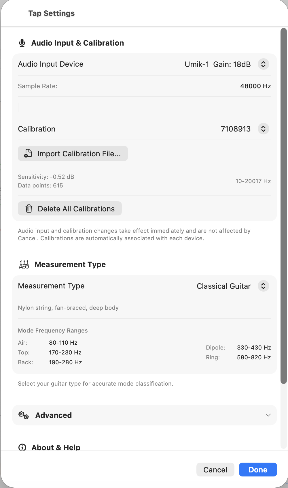
2.5 Choosing a Measurement Type
In Settings, the Measurement Type section determines what the analyzer is looking for:
- Generic Guitar / Acoustic Guitar / Classical Guitar / Flamenco Guitar. Guitar-body mode. The four sub-types differ in the expected frequency windows for the air, top, back, and dipole modes; pick the one closest to the instrument you are measuring. Generic uses the broadest windows.
- Plate. Free-plate measurement with the longitudinal, cross-grain, and optional free-length-cross phases.
- Brace. Single-tap longitudinal measurement on an individual brace.
The choice persists across launches. Changing it mid-sequence starts a new sequence in the new mode.
2.6 Setting the Threshold — Finding Your Tap Level
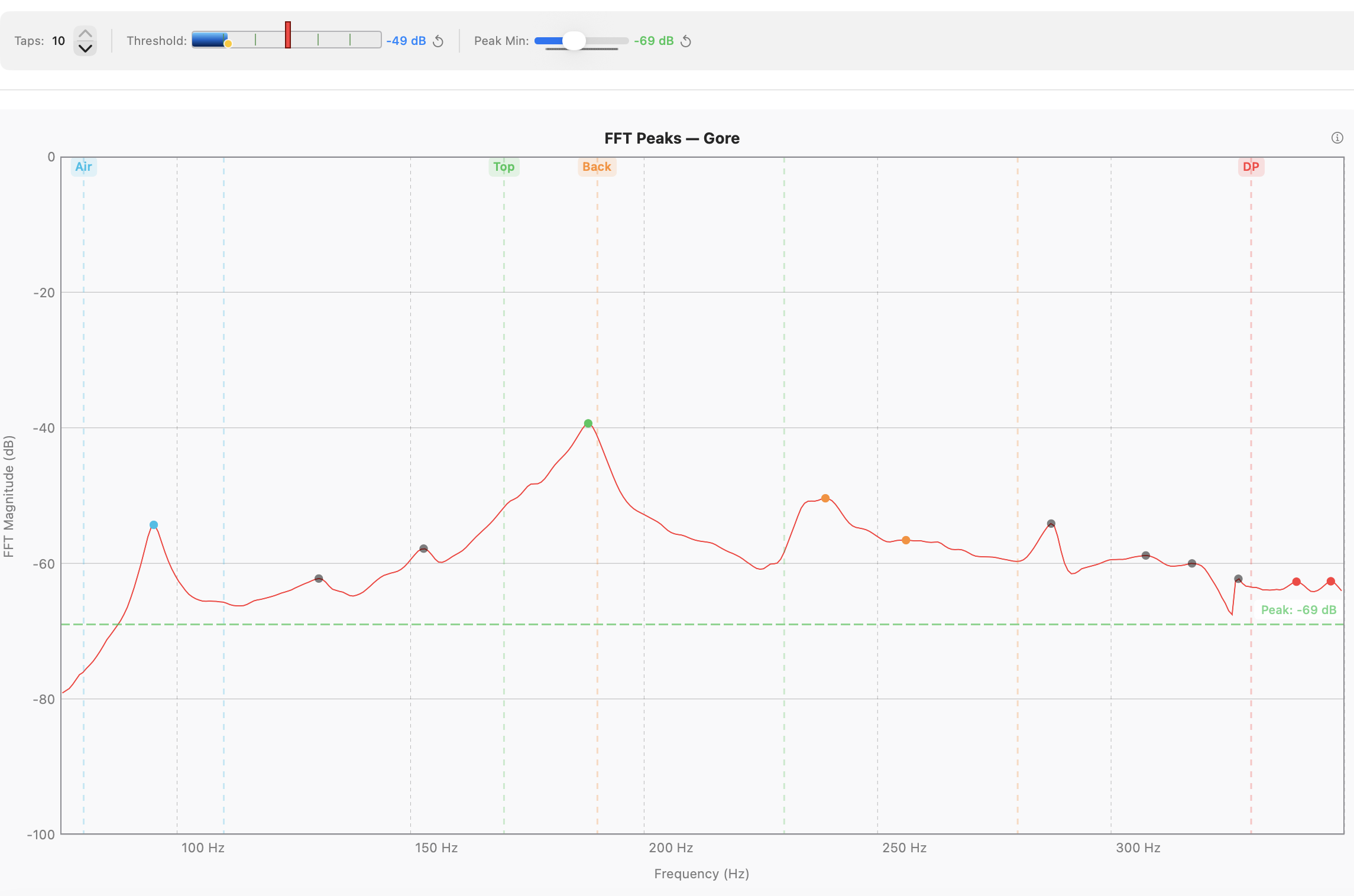
The Threshold slider sets the signal level a tap must exceed before the analyzer captures it. You will tune it once for your microphone, room, and tapping style; the value then persists.
The tuning procedure is the same in all three measurement modes:
- Press Pause. The spectrum stays live, but no taps will register — you can experiment without triggering a measurement.
- Make a representative tap and read the highest dB the live spectrum reaches.
- Set Threshold roughly 6 to 10 dB below that peak level. This leaves headroom for tap-to-tap variation while staying clear of ambient noise.
- Press Resume and tap again. The spectrum should freeze and the Tap Detected indicator should appear.
If taps are missed, lower the threshold. If ambient noise triggers false captures, raise it.
2.7 Setting Peak Min — Filtering the Peak List (Guitar Mode)
Peak Min sets the minimum spectrum magnitude at which a peak is annotated on the chart and considered for guitar-mode analysis. It is a guitar-mode control: in Plate and Brace modes the per-phase capture uses its own adaptive noise floor, and Peak Min only affects which peaks are drawn — never which are selected for the calculation.
Tune it from the same paused state used for Threshold:
- Still paused (continuing from §2.6), make a few representative taps and watch the peaks appear on the live spectrum.
- Raise Peak Min until noise peaks disappear. Lower it until the structural resonances you care about are visible.
- Press Resume and take the real measurement.
If you adjust Peak Min on a frozen spectrum after a measurement, press the wand button to re-run automatic mode selection against the new threshold.
Peak Min persists across launches.
2.8 Your First Tap — Guitar Mode Walkthrough
You now have everything you need.
- Position the microphone 5 to 15 cm from the sound hole. (For top- or back-tap measurements, position it 5 to 10 cm from the tap point.)
- The analyzer is already running on launch. Confirm Threshold and Peak Min are tuned per §2.6 and §2.7.
- Press Resume if you paused during tuning. The detector is armed and the spectrum is live.
- Tap the guitar — a knuckle rap on the bridge or a bouncy-ball strike on the back, depending on what you are measuring. The spectrum freezes when the tap registers.
- Open the Analysis Results panel and review the identified modes, frequencies, ring-out time, and tap-tone ratio.
- Press Save in the top toolbar to store the measurement so you can compare it to future taps.
That is a complete cycle. From here, see the use-case chapters for the workflow you actually want to run — guitar (Chapter 3), plate (Chapter 4), or brace (Chapter 5).
Chapter 3 — Guitar Mode
Guitar mode captures the body resonances of a completed instrument and presents them as a labelled peak list. This chapter assumes the microphone, calibration, threshold, and peak-min are already tuned as described in Chapter 2.
3.1 Mode Labels and Classification
Guitar Tap identifies and labels six classes of guitar-body modes: Air, Top, Back, Dipole, Ring, and Upper Modes. Classification is by frequency window: each guitar subtype (Generic, Acoustic, Classical, Flamenco) defines a range of frequencies in which a candidate for each mode is expected. The strongest peak inside a window is assigned to that mode; peaks outside every window are labelled Unknown.
Unknown peaks are shown on the chart by default so nothing in the spectrum is silently hidden. If you find them cluttering a chart that you intend to share or compare, turn them off via Settings → Advanced → Analysis Settings → Show Unknown Modes.
Generic is the recommended subtype for most measurement work. Its windows are wide enough to catch the air, top, and back modes of any of the common guitar archetypes, which is what you want when you simply need to see and label the resonances of the instrument in front of you. The other subtypes — Acoustic, Classical, Flamenco — are narrower and are most useful when:
- you want the quality indicators in the Results panel to reflect the typical frequency band for that style (the colour cues next to each mode and the tap-tone ratio are interpreted against the chosen subtype's expectations); or
- you are building or voicing to a target frequency range associated with a particular style and want the windows to exclude peaks that fall outside that target.
The frequency windows can be inspected in Settings → Measurement Type when a subtype is selected.
3.2 Setting Up for Guitar Mode
- Open Settings → Measurement Type and choose Generic Guitar unless you have a specific reason (quality indicators or a target frequency range) to choose Acoustic, Classical, or Flamenco — see §3.1.
- The frequency-window panel updates to show the ranges for the selected subtype. Confirm they bracket the modes you expect to find.
- Show Unknown Modes is on by default. Leave it on unless you are preparing a chart for sharing and want to declutter.
- Confirm Threshold and Peak Min are tuned for the current mic and room (see §2.6 and §2.7).
3.3 Microphone Placement
- Distance: 5 to 15 cm from the sound hole for body-cavity measurements; 5 to 10 cm from the tap point for top or back measurements.
- Angle: roughly perpendicular to the soundboard or back, but not so close that the diaphragm sees only one localized region.
- Surroundings: avoid hard surfaces within ~30 cm of the microphone. Reflections add spurious peaks and inflate the noise floor at the comb frequencies of the workbench geometry.
- Reproducibility: mark the mic position (a piece of tape on the bench is sufficient) if you intend to compare measurements across sessions on the same instrument. Small position changes shift the relative magnitudes of modes you may want to track build-to-build.
3.4 Single Tap Measurement
- Press New Tap to arm the detector. The status area shows the analyzer is waiting for a tap.
- Tap the instrument: a short, crisp knuckle or fingertip rap on the bridge, or a bouncy-ball strike on the back.
- The Tap Detected indicator appears and the spectrum freezes automatically.
- Read the annotated peaks on the frozen spectrum and the Analysis Results panel (see §3.8 for what each column means).
If the tap was missed or contaminated (a finger squeak, an ambient transient), press New Tap again to discard it and try once more.
If Threshold or Peak Min need adjusting before the live take, press Pause first — the spectrum stays live and no taps will register while you experiment. Move the sliders, tap freely, then press Resume when ready.
3.5 Multi-Tap Averaging
For tighter results, average several taps in one sequence.
- Set the Taps stepper at the top of the toolbar to the number of taps you want (1 to 10). Five is a common choice.
- Press New Tap as before. The status bar now shows progress — "Tap 1/5", "Tap 2/5", and so on.
- Tap the instrument the required number of times. Each captured tap re-arms the detector after a short cooldown; the spectrum re-freezes only after the final tap.
- When all taps are captured, the averaged spectrum is displayed with annotated peaks. Individual tap spectra are retained for comparison (see §6.x for the multi-tap comparison view).
Pause between taps. Press Pause if you need to pause mid-sequence (to reset the instrument's position, for example). The captured taps so far are preserved; Resume continues from where you left off.
Cancel mid-sequence. Press Cancel to discard all captured taps and end the sequence. New Tap then re-arms for a fresh attempt.
3.6 Inspecting and Adjusting Peak Selections
Each peak in the frozen spectrum is shown with a label (mode name) and a coloured dot whose colour matches its row in the Analysis Results panel.
- Toggle a peak's selection by tapping its label on the chart. Selected peaks contribute to derived values such as the tap-tone ratio; deselected peaks remain visible but are excluded from the calculation.
- Cycle the annotation set using the Annotations button: All (every detected peak labelled), Selected (only currently selected peaks), or None (no labels on the chart). The default is Selected, which matches what most luthiers want to see.
- Re-run automatic selection by pressing the wand button in the Analysis Results header. This is useful after raising or lowering Peak Min on a frozen spectrum: the wand re-classifies the visible peaks against the current Peak Min and re-selects one per mode window.
- Select All / Select None are available in the Results header for the cases where you want everything on or off in one step.
Selection changes are preserved when the measurement is saved.
3.7 Overriding Mode Classification
The automatic classifier occasionally picks the wrong peak — for example, when two candidates are close in magnitude and the wrong one falls inside the configured window. To correct it:
- In the Analysis Results panel, tap the row of the peak whose label you want to change.
- A mode picker appears with Air, Top, Back, Dipole, Ring, Upper Modes, Unknown, and a Custom label field for free-text annotations.
- Pick the correct mode. The chart label updates immediately.
Overrides are saved with the measurement and reapplied when the measurement is loaded later. The wand button respects manual overrides — a re-classify will not silently undo your choice.
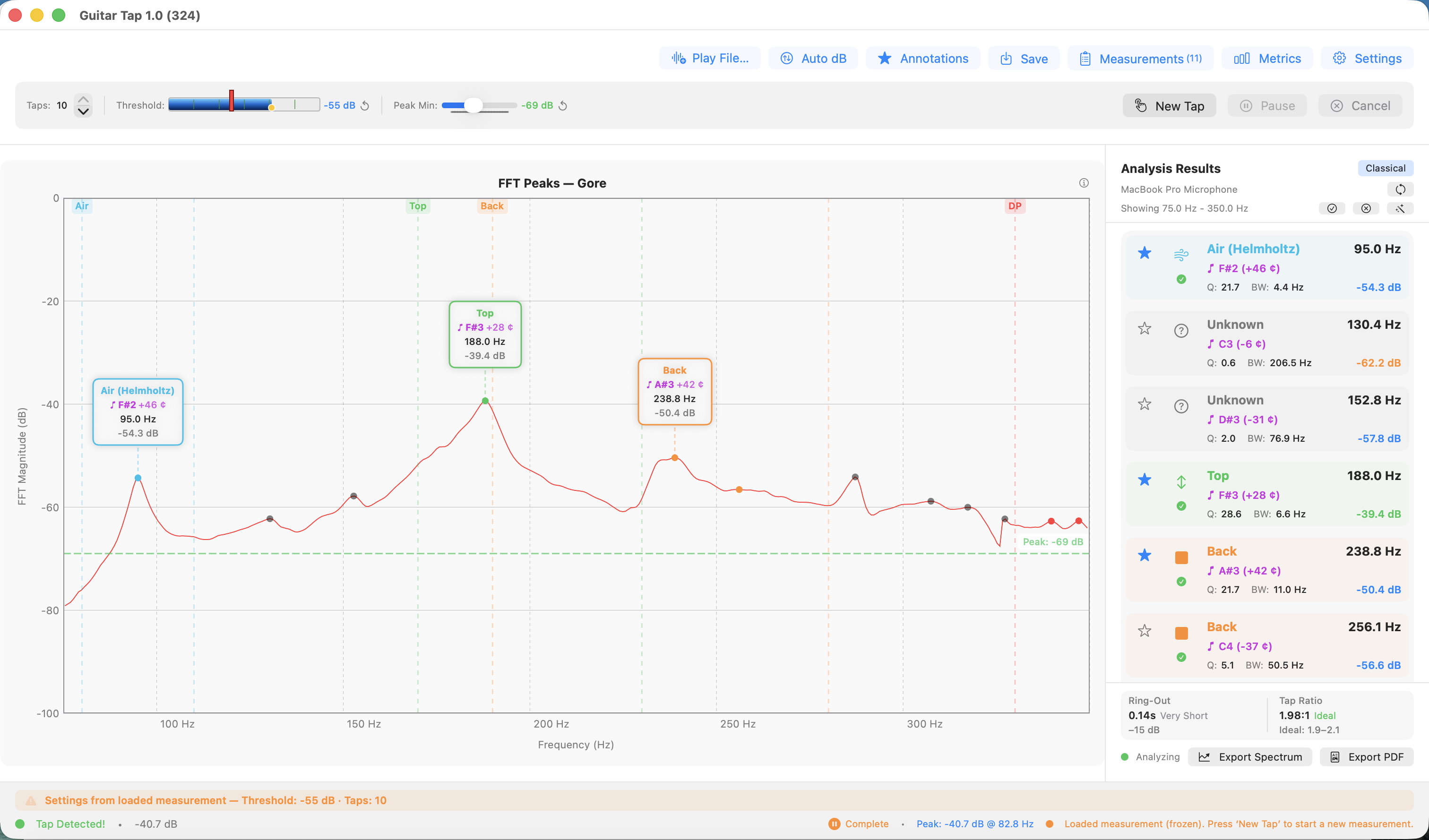
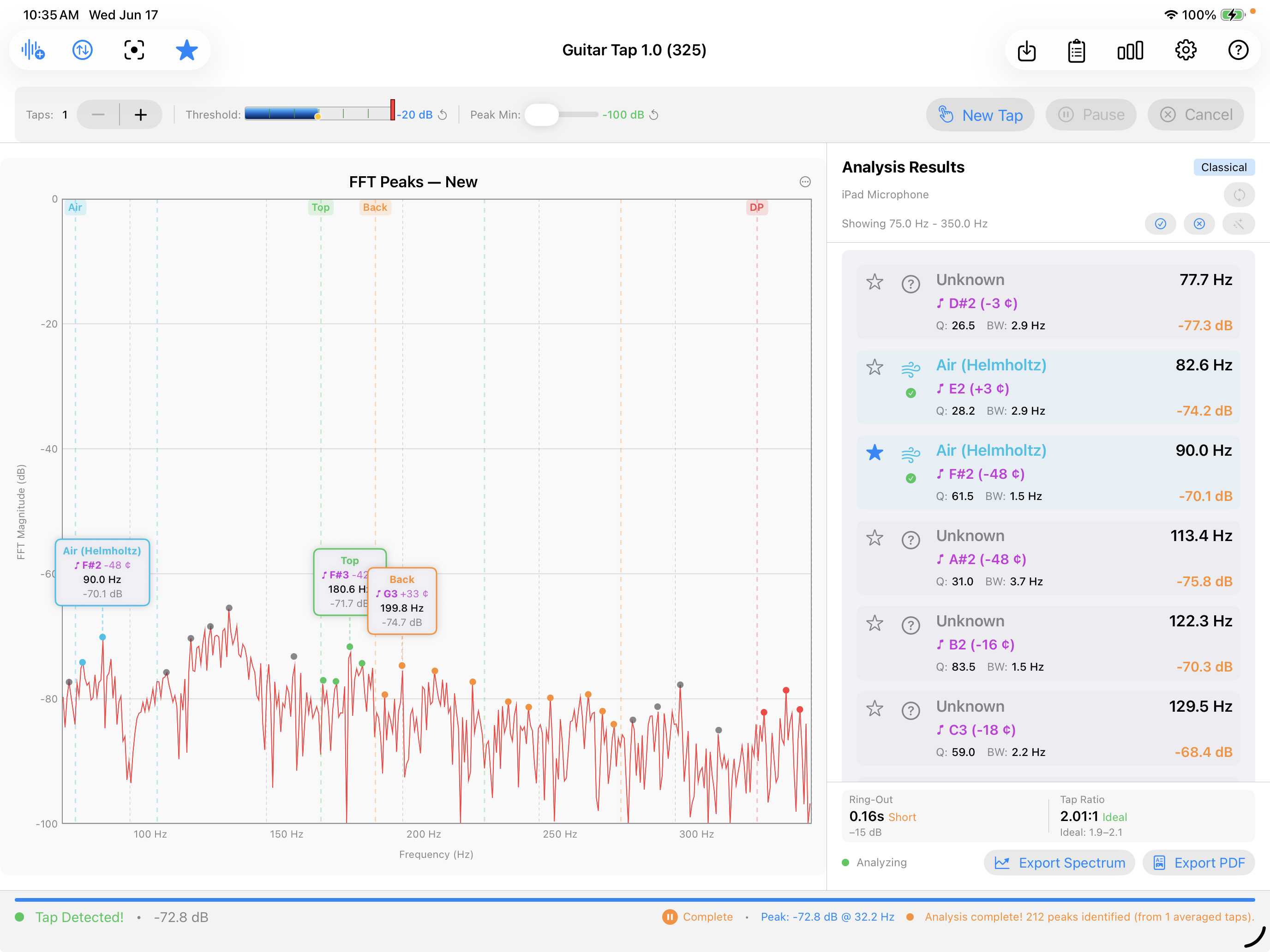
3.8 Reading the Results Panel
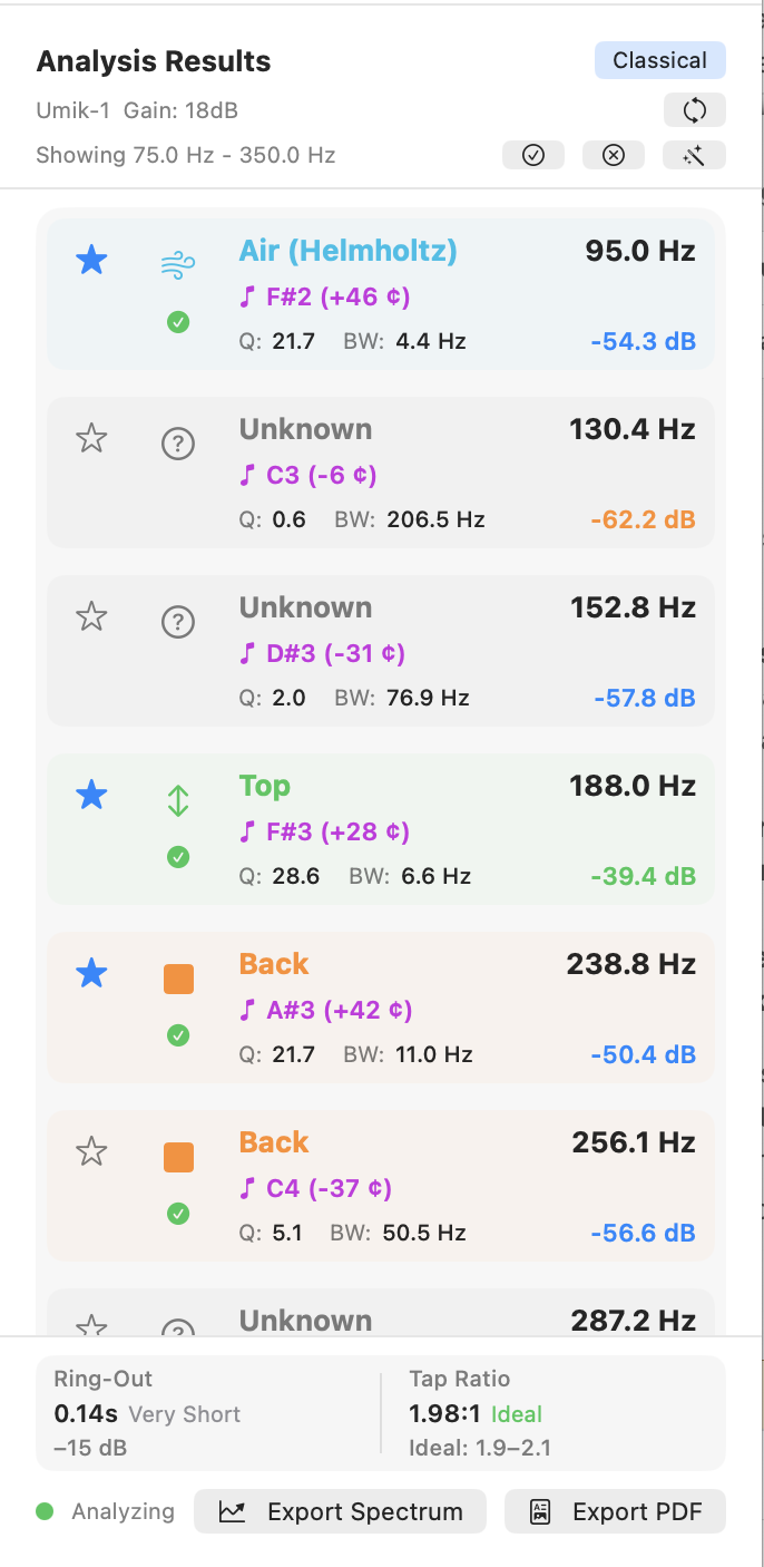
For each identified peak the Analysis Results panel shows:
- Mode label — Air, Top, Back, Dipole, Ring, Upper, or a custom override.
- Frequency — in Hz, to 0.1 Hz.
- Magnitude — in dB, relative to the spectrum's reference.
- Q — quality factor (centre frequency ÷ −3 dB bandwidth).
- Bandwidth — −3 dB bandwidth in Hz.
- Pitch — nearest equal-temperament note plus cents offset.
Below the peak list:
- Ring-out — decay time in seconds, computed from the magnitude envelope after the tap impulse. A structural-damping indicator.
- Tap Tone Ratio — f_Top ÷ f_Air. Typical values for a well-voiced guitar fall in the 1.8–2.4 range; the value is shown with a colour cue indicating whether it is in, near, or outside that band.
When a value is missing (a mode was not identified, or the ring-out could not be measured), the panel displays "—" rather than zero so the absence is unambiguous.
3.9 Comparing Guitar Measurements
Comparison overlays two to five saved guitar measurements on the same chart. Useful for any pair-or-more of measurements you want to see side by side — different build stages of the same instrument, different tap locations on the same body, different instruments you have built, or measurements of instruments built by someone else that you want to study or learn from.
Starting a comparison
- Open the Measurements list.
- Tap to select two to five saved guitar measurements. Plate and brace measurements are excluded — comparison is guitar-only.
- Tap the Compare button that appears once two or more measurements are selected.
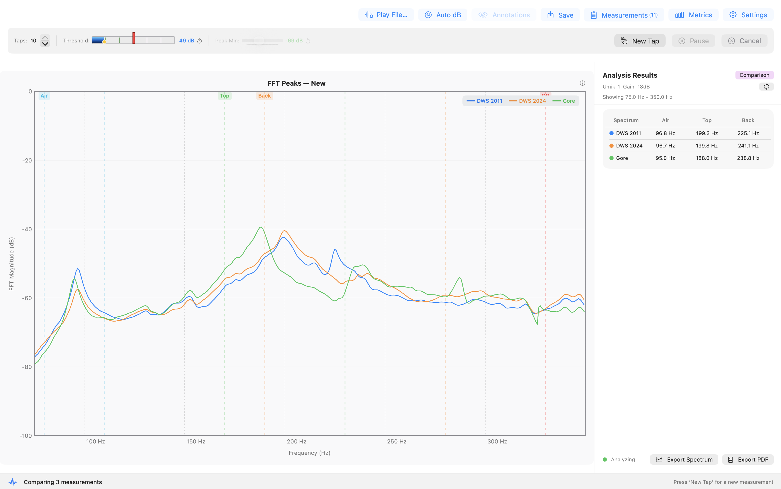
The chart switches to comparison view: each selected spectrum is drawn in a distinct colour with a legend. The Analysis Results panel switches to a comparison table with one column per spectrum (labelled with the colour dot from the legend) and rows for Air, Top, and Back frequencies. "—" appears where a mode was not identified.
What is available during comparison
Save, Export Spectrum, and Export PDF Report all remain active, but they operate on the overlay rather than on an individual measurement:
- Save stores the entire overlay as a single comparison in the Measurements list. The save sheet accepts an optional location label and notes. The saved comparison appears with a distinct badge and can be reloaded later to restore the overlay — every spectrum, its colour, and the Comparison Results table — exactly as it was.
- Export Spectrum (⌘E on macOS; Ctrl+E on Windows / Linux) writes an overlay PNG with all curves, their colours, and the legend.
- Export PDF Report (⇧⌘E on macOS; Ctrl+Shift+E on Windows / Linux) writes a comparison PDF: a metadata header (number of spectra, labels, date), the overlay image, and an Air / Top / Back frequency table with one column per spectrum.
A saved comparison .guitartap file can be imported via
File → Import Measurement (macOS / Python desktop) or the
Import Measurement button in the Measurements list (iOS). The app
detects the comparison on load and restores the overlay.
What is inactive during comparison
- Annotations button — each spectrum carries its own annotations set at capture time; there is nothing to cycle in the overlay.
- Threshold and Peak Min sliders — the comparison view is a static overlay of frozen measurements; live detection is not running.
- Taps stepper — no active capture sequence to configure.
Exiting comparison. Press New Tap to leave comparison mode and return to single-measurement operation.
Chapter 4 — Plate Mode
Plate mode captures the longitudinal, cross-grain, and (optionally) free-length-cross resonances of a rectangular tonewood blank and returns the moduli, specific modulus, radiation ratio, and Gore target thickness for the piece. This chapter assumes the microphone, calibration, threshold, and peak-min are already tuned as described in Chapter 2.
4.1 Overview of Plate Material Measurements
Plate mode runs a guided sequence of two or three taps on a rectangular blank suspended at its nodal points and computes the material properties used to evaluate a piece of tonewood:
- Longitudinal (L) — bending mode with grain. Yields E_L and c_L.
- Cross-grain (C) — bending mode across the grain. Yields E_C and c_C.
- Free-length-cross (FLC) — torsional mode, optional. Yields the shear modulus G_LC, which feeds the Gore target thickness calculation and tightens its result by roughly 5 to 7%.
From these the app derives ρ (from your dimensions and mass), specific modulus E_L/ρ, radiation ratio R, the E_C/E_L cross-to-long ratio, a quality rating against the spruce scale, and the Gore target thickness for the body dimensions and stiffness preset you have selected.
Plate mode is for raw blanks before bracing or cutting. For an individual brace, use Brace mode (Chapter 5); for a finished body, use Guitar mode (Chapter 3).
4.2 Preparing the Sample
The blank should be a clean rectangle with the grain parallel to one long axis. The numbers you enter into the app drive every derived quantity, so accuracy matters:
| Field | Target accuracy |
|---|---|
| Length (along grain) | 0.5 mm |
| Width (cross grain) | 0.5 mm |
| Thickness | 0.1 mm |
| Mass | 0.1 g |
A digital caliper handles the thickness measurement. Length and width are typically beyond the jaw span of a caliper for guitar-scale blanks; an accurate steel rule is the better tool there. A jeweller's scale or any 0.1 g kitchen scale handles mass.
Mass error dominates. Length and width errors scale linearly into the moduli; thickness scales as the cube. A 1% mass error and a 0.3% thickness error produce comparable changes in E.
4.3 Entering Dimensions in Settings
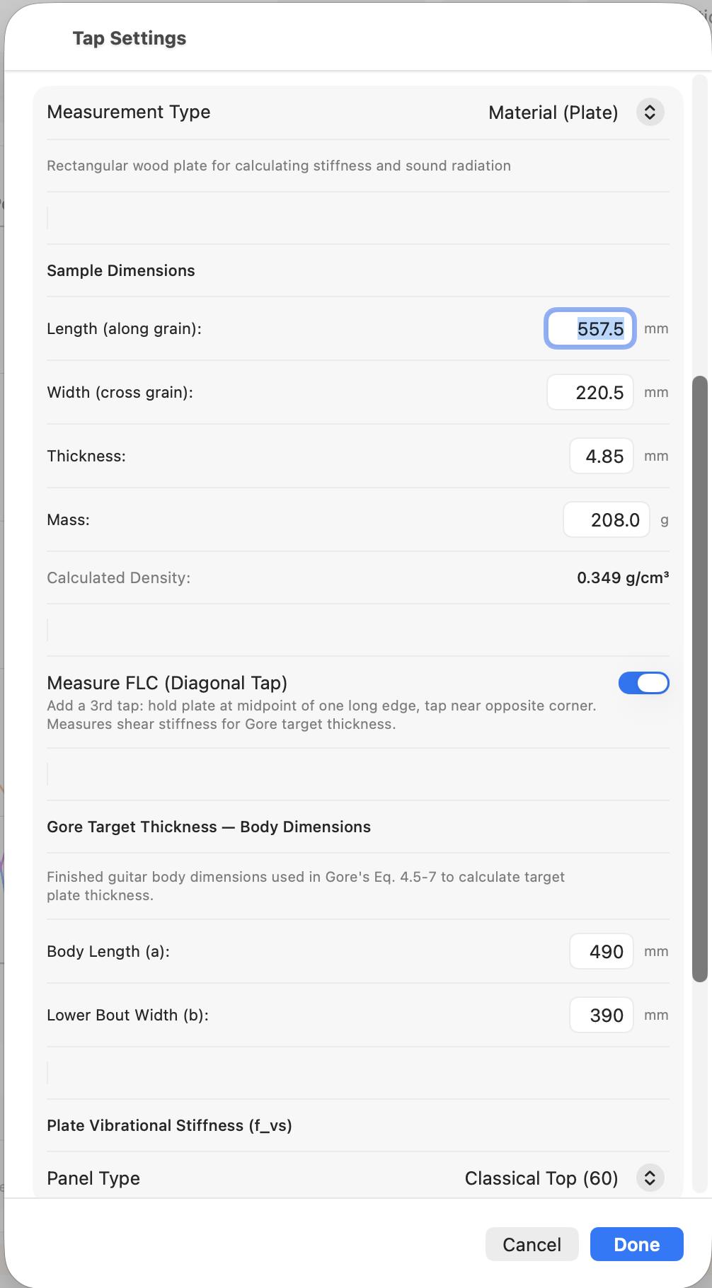
Open Settings → Measurement Type → Plate. Fill in:
- Length (mm) — along the grain.
- Width (mm) — across the grain.
- Thickness (mm).
- Mass (g).
A live density preview appears below the dimension fields. Use it as a sanity check on data entry. Spruce typically lands in the 0.35–0.45 g/cm³ band; a value below 0.30 or above 0.70 is almost always a transposed digit or a unit error somewhere in the four fields.
For the Gore target thickness, also enter:
- Body Length (mm) and Lower Bout Width (mm) — the dimensions of the instrument the plate is destined for.
- Plate Stiffness Preset — the target stiffness number the Gore
thickness calculation solves for. The named presets are starting
points calibrated to typical instrument styles:
- Steel String Top (75)
- Steel String Back (55)
- Classical (50)
- Custom — accepts any numeric target.
Custom is where you encode a successful build back into the calculation. The workflow has four steps:
- Fully measure a plate — E_L, E_C, density, body dimensions — before you build it, and keep the measurements. Note the final plate thickness you settled on for the build (which may be the number from the Gore formula).
- Build the instrument and live with it long enough to decide whether the result is what you want. If it is, you have a calibration point. If not, you need to adjust the plate stiffness preset on your next build to either stiffen the board or loosen it to adjust the sound.
- The Gore formula run on that plate's measurements with a named preset would have predicted some recommended thickness. Your finished thickness is the thickness that actually produced the sound you liked. Scale the preset's stiffness number linearly so the formula, applied to that same plate's measurements, would output your finished thickness. Save the scaled number as your Custom value.
- From this point on, run new plates with Custom selected. Each new board, with its own E_L, E_C, and ρ, yields a different recommended thickness — each one calculated to reproduce the calibration build's tonal outcome on that specific piece of wood.
The Custom number carries "this is the kind of plate that makes the instrument I want." The Gore procedure does not predict an objectively ideal thickness; it gives you a reproducible way to translate a tonal target across pieces of wood that differ in stiffness and density.
Measure FLC is a toggle in the same section. Turn it on if you intend to capture the FLC tap (§4.8). The sequence then runs in three phases instead of two.
4.4 The 22% Suspension Technique
The three taps share one principle: hold the blank at a nodal point of the mode you want to measure, and tap at an antinode.
For longitudinal and cross-grain there is a catch — both modes are easy to excite at the same time, and the hold point alone decides which one wins in the spectrum. A hold on a mode's nodal line suspends that mode (it can vibrate freely); a hold on a mode's antinode damps it. To get a clean reading the hold must sit on the target mode's node and off the orthogonal mode's node.
In all three orientations the tap point is the centre of the plate face.
-
Longitudinal. Plate oriented with grain horizontal.
- The longitudinal mode's nodal line runs cross-wise at 22% from each short end.
- The cross-grain mode's nodal lines run length-wise at 22% from each long edge.
- Hold between thumb and forefinger 22% in from one short end along the length, close to one long edge but not at 22% in from it. The other end of the plate hangs free; tap at the centre.
-
Cross-grain. Rotate the plate 90° so grain is now vertical. Same logic with the modes swapped: now the cross-grain mode's node is the one you want to be on, and the longitudinal mode's node is the one to avoid.
- Hold 22% in from one long edge, close to one short end but not at 22% in from it. Other end hangs free.
-
FLC. One hand only. Hold at the midpoint of one long edge. Tap near the opposite corner, approximately 22% in from both the end and the side. The torsional mode FLC excites has its node along the centreline of the plate, so a single midpoint hold is enough.
Common errors: putting the hold on both modes' node lines at once (contamination — a longitudinal reading that looks like cross-grain or vice versa); holding too far in along the target axis (the support falls inside the mode shape and damps it); holding too firmly (adds damping regardless of position); and forgetting to rotate the plate between L and C — easy to do, easy to spot when C reads close to L.
4.5 The Accept / Redo Review Flow
Plate mode runs each phase as: arm, tap, freeze, review.
After a tap is captured the spectrum freezes and the detector pauses automatically. The tap controls re-label for the review state:
- The Pause button becomes Accept (green tint, checkmark icon). Pressing it locks in the current phase result and advances to the next phase. The next phase arms detection on its own — you do not need to press New Tap between phases.
- The Cancel button becomes Redo (orange, labelled Redo L, Redo C, or Redo FLC depending on which phase is being reviewed). Pressing it discards the current phase result and re-arms detection for the same phase.
During review the live spectrum is suppressed so the captured spectrum stays on screen for inspection. The status bar shows the current phase and tap count: Phase 2/3 · Tap 1/1, for example.
After every phase is accepted the Results panel updates with the complete plate calculations (§4.9).
Individual phase redo is only available before that phase is accepted. To restart the entire sequence — for example, you realise mid-FLC that the longitudinal tap was made before you'd entered the right dimensions — press New Tap; the captured phases are discarded and the sequence starts again from Longitudinal.
4.6 Tap 1 — Longitudinal
- Orient the plate with the grain running horizontally.
- Hold at 22% from each end along the length, near one long edge.
- Press New Tap. The status bar shows Capturing Longitudinal · Phase 1/2 (or Phase 1/3 if Measure FLC is on).
- Tap the centre of the plate face.
- The spectrum freezes. Inspect the lowest peak — it should be the longitudinal bending mode for a free-free beam of your dimensions, typically in the low hundreds of Hz for a guitar top.
- Press Accept to lock the phase in, or Redo L to re-capture if the tap was contaminated.
After Accept the sequence advances to Cross-grain automatically.
4.7 Tap 2 — Cross-Grain
- Rotate the plate 90° so the grain now runs vertically.
- Hold at 22% from each end along the width, near one short edge.
- The status bar now reads Capturing Cross-grain · Phase 2/2 (or Phase 2/3). Detection is already armed — do not press New Tap.
- Tap the centre of the plate face.
- Inspect the frozen spectrum, then Accept or Redo C.
After Accept, the sequence either advances to FLC (if Measure FLC is on) or marks the measurement complete.
4.8 Tap 3 — FLC (Optional)
FLC measures the flat long/cross torsional mode and yields the shear modulus G_LC. The Gore target thickness calculation uses G_LC for its shear correction; without it, the calculation substitutes a default that over-estimates target thickness by roughly 5 to 7%. For final plate thicknessing, capturing FLC is worth the extra tap.
- Enable Measure FLC in Settings before starting the sequence if you have not already.
- Hold one long edge at its midpoint, with one hand only.
- The status bar reads Capturing FLC · Phase 3/3.
- Tap near the opposite corner, approximately 22% in from the end and 22% in from the side.
- Accept or Redo FLC.
After Accept the measurement is complete and the Results panel updates with Gore target thickness including the shear correction.
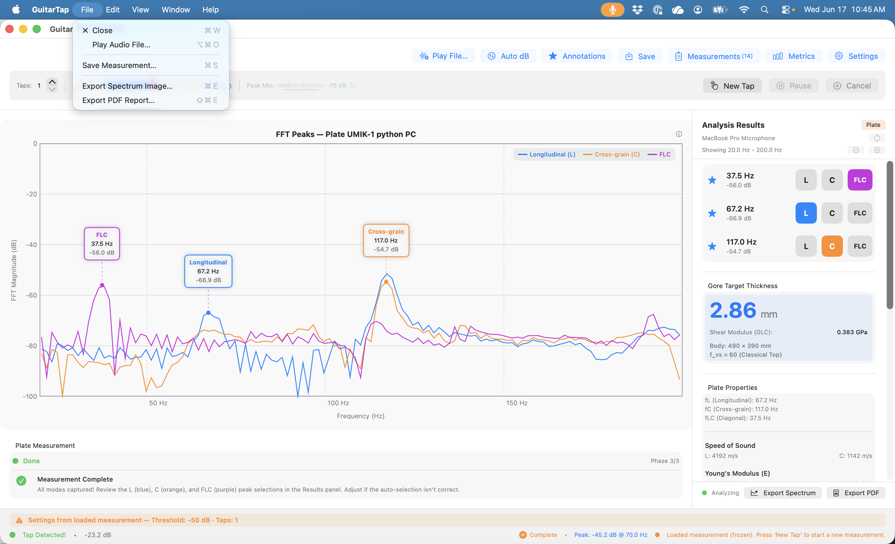
4.9 Reading Plate Results
For a completed plate measurement the Results panel scrolls through four sections, top to bottom.
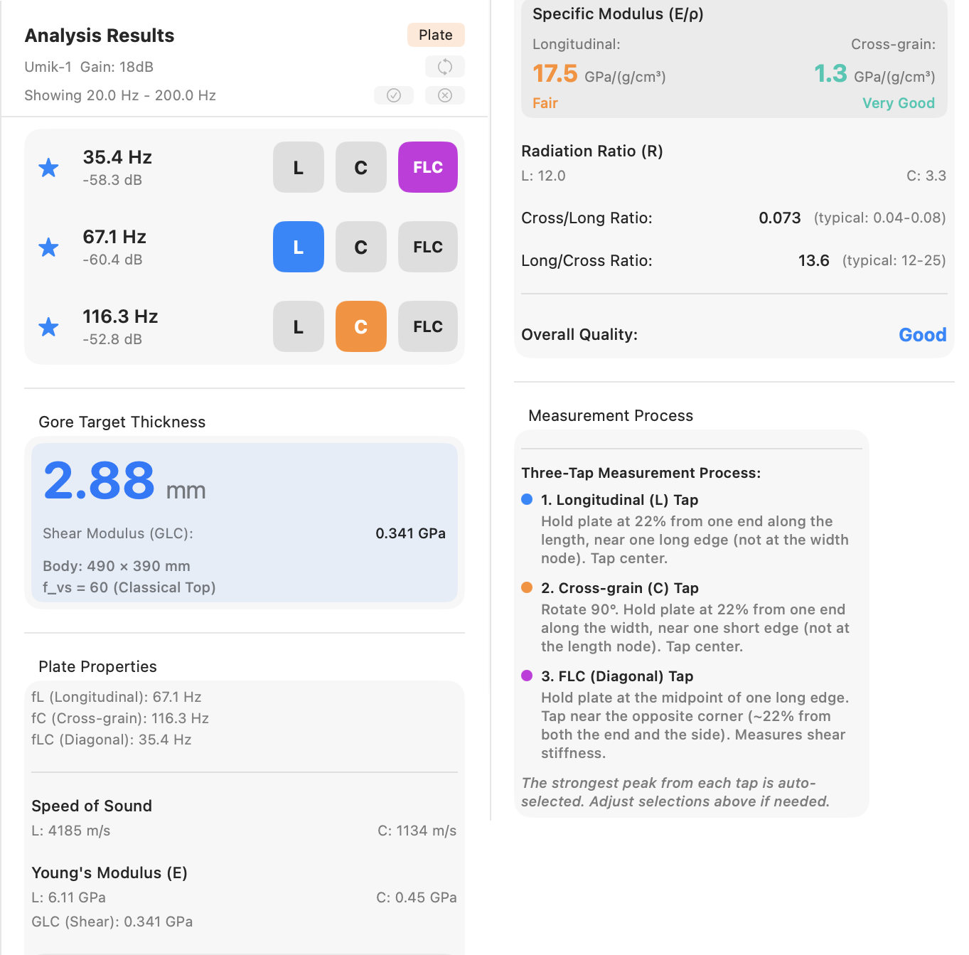
Detected Peaks
One row per captured phase — two rows (L, C) for a two-tap sequence, three rows (L, C, FLC) when FLC is enabled. Each row shows a selection-indicator star, the peak frequency, the peak magnitude in dB, and a coloured phase badge identifying which mode the peak belongs to (blue L, orange C, purple FLC). The full detected-peak list and the Peak Min filter from guitar mode do not apply here; what you see is the auto-selected best peak from each phase capture.
Gore Target Thickness
The headline thickness for the body dimensions and stiffness preset entered in Settings, displayed prominently in mm. Below the number:
- Shear Modulus (G_LC) — the value used in the thickness calculation, shown when FLC was measured.
- "G_LC assumed 0 — enable FLC tap for a more accurate result" — shown when FLC was skipped. The thickness above is then approximate (roughly 5 to 7% over-estimate; see §4.8).
- Body dimensions and the f_vs value (with preset name, or a literal "custom" annotation when Custom is active) — the parameters that fed the calculation, exposed so you can cross-check Settings against the body the plate is destined for.
Plate Properties
Material characterisation of the wood:
- Frequencies used — fL, fC, and (if measured) fLC.
- Speed of Sound — c_L and c_C in m/s.
- Young's Modulus (E) — E_L and E_C in GPa. G_LC is appended to this block when FLC was measured; the row is absent when FLC was skipped.
- Specific Modulus (E/ρ) — the headline material number, in GPa/(g/cm³). Shown in large type for both Longitudinal and Cross-grain, each with a per-direction quality rating (Excellent / Very Good / Good / Fair / Poor against the spruce scale) and a colour cue matching that rating.
- Radiation Ratio (R) — reported for both directions.
- Cross/Long Ratio — E_C / E_L. Typical spruce 0.04 to 0.08; the typical band is shown beside the value.
- Long/Cross Ratio — the reciprocal. Typical spruce 12 to 25; the typical band is shown beside the value.
- Overall Quality — a separate row at the bottom of the section combining both directions into a single rating (Excellent / Very Good / Good / Fair / Poor) with the matching colour cue.
The quality scales are calibrated for spruce; readings on cedar, redwood, or other top woods read as a point of comparison rather than an absolute grade.
Plate Process Instructions
A reference card describing the two-tap (or three-tap, if FLC is enabled) measurement procedure. Useful as an in-place refresher when you come back to plate mode after a break and want the hold and tap positions without leaving the results panel.
4.10 Interpreting Plate Results
Specific modulus and radiation ratio capture what Young's modulus alone misses: how stiff a plate is per unit of weight it is asking the player to drive. Two blanks with identical E_L can sit in very different quality bands when their densities differ. Sort by E_L/ρ, not E_L, when triaging a stack of blanks.
Gore target thickness is a starting point for thicknessing, not a specification. Reproduce it on the bench, then voice from there with hands-on tap-tone evaluation; the final number lives at the intersection of your wood, your bracing pattern, and the instrument design you are building toward.
For tracking measurements across multiple blanks: enter a brief identifier (board number, supplier, billet) into the Notes field on the Save sheet so the saved measurement carries its provenance. Plate measurements can be saved, reloaded, and exported the same way guitar measurements can (Chapter 7); the comparison overlay described in §3.9 is guitar-only.
Chapter 5 — Brace Mode
Brace mode is a fast, single-tap longitudinal measurement for an individual brace strip. It reports the moduli, specific modulus, and quality rating in one capture; cross-grain, shear, and Gore thickness are all skipped. This chapter assumes the microphone, calibration, threshold, and peak-min are already tuned as in Chapter 2.
5.1 Overview
Brace mode runs a single longitudinal tap on a brace strip and returns the wood's stiffness and quality. Compared to Plate mode:
- No cross-grain tap. E_C is not measured.
- No FLC tap. G_LC is not measured.
- No Cross/Long ratio.
- No Gore target thickness. Brace mode is for stock evaluation, not for thicknessing.
What you get: E_L, c_L, specific modulus E_L/ρ with a per-direction quality rating against the spruce scale, and radiation ratio R.
Brace mode is intended for batch-evaluating brace strips before selecting stock for a build. For a free plate, use Plate mode (Chapter 4); for a complete instrument, use Guitar mode (Chapter 3).
5.2 Setting Up Brace Dimensions
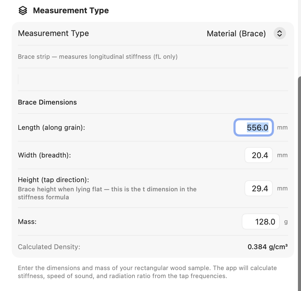
Open Settings → Measurement Type → Brace. The Brace Dimensions section has four fields:
- Length (along grain) (mm) — the long axis of the strip.
- Width (breadth) (mm) — the brace's breadth lying flat.
- Height (tap direction) (mm) — the dimension perpendicular
to the face you tap. This is the
tin the Euler–Bernoulli stiffness formula, so it's the one that drives E_L most strongly. The Settings panel itself flags this with a helper line under the field; double-check it before tapping. - Mass (g).
A Calculated Density line appears below the fields once all four are populated. Use it the same way as the plate-mode density preview — spruce should land in the 0.35–0.45 g/cm³ range, and a value well outside that is almost always a digit transposition.
5.3 Technique
A brace strip is a long thin beam — the same free-free fundamental applies, but the measurement is much simpler than plate because only one mode is in play.
- Hold the strip between thumb and forefinger 22% in from one end along the length. The other end hangs free.
- Lay the strip flat (or mount it however you usually orient it
on the bench) so the face you intend to tap is exposed. The
Heightvalue in Settings must match the dimension perpendicular to this face. - Press New Tap.
- Tap the centre of the top face. The spectrum freezes when the tap registers.
The Accept / Redo review flow is the same as in Plate mode (see §4.5). Accept locks in the measurement; Redo discards it and re-arms the detector. There is no phase counter — Brace mode runs in a single phase, so the status bar shows just the current state.
5.4 Reading Brace Results
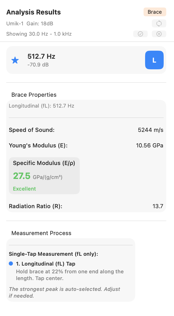
A completed brace measurement displays three sections in the Results panel.
Detected Peaks
A single row for the longitudinal peak. It shows a selection-indicator star, the peak frequency, the peak magnitude in dB, and a blue L phase badge.
Brace Properties
- Frequency used — fL in Hz.
- Speed of Sound — c_L in m/s.
- Young's Modulus (E) — in GPa.
- Specific Modulus (E/ρ) — the headline number, in GPa/(g/cm³), shown in large type. A quality rating (Excellent / Very Good / Good / Fair / Poor against the spruce scale) accompanies the value with a matching colour cue.
- Radiation Ratio (R) — in the same column.
There is no Cross/Long ratio or Overall Quality row — both are plate-only since they need cross-grain data.
Brace Process Instructions
A reference card describing the brace measurement procedure. Useful as an in-place refresher when you have come back to Brace mode after a break.
5.5 Using Brace Mode to Compare Stock
A practical workflow for evaluating a batch of brace strips:
- Label each strip (a pencil mark on the end grain or a small sticky label works) so you can match measurements to physical pieces later.
- Enter the strip's Length, Width, Height, and Mass in Settings. For a batch of strips with consistent stock dimensions you only have to change Mass between measurements; for variable stock all four fields need updating.
- Tap the strip.
- Record the result. The Notes field on the Save sheet is the right place for the strip's identifier — once saved, the saved measurement carries its provenance.
- Move on to the next strip.
For sorting by stiffness alone, the longitudinal frequency at the same dimensions is a sufficient proxy — higher fL means stiffer stock. For triaging across different sizes, sort by specific modulus (E_L/ρ).
A practical limitation worth keeping in mind: with no cross-grain or shear data, brace-to-brace comparisons are one-dimensional. A strip that reads well in brace mode might still have anisotropy or grain runout that only shows up in a plate-style measurement on the parent billet.
Chapter 6 — Working with the Spectrum
The spectrum chart is the centrepiece of the analysis screen. This chapter covers the gestures, shortcuts, and settings that let you read it the way you want without disturbing the measurement itself.
6.1 Live vs. Frozen Spectrum
Before a tap registers, the spectrum is live — the chart redraws on every FFT frame, showing the current microphone input in real time. Use this state to monitor ambient noise, dial in Threshold and Peak Min while paused (§2.6, §2.7), or simply confirm the microphone is working.
When a tap registers, the spectrum freezes on the capture so you can inspect peaks, drag labels, and read the Analysis Results panel without the chart moving under you. The status bar shows "Tap Detected" when the freeze happens.
Pressing New Tap discards the frozen capture (or current sequence) and returns to live mode, arming the detector for the next tap.
6.2 Zooming and Panning — iOS and iPadOS
- Pinch anywhere over the plot area to zoom both axes.
- Pinch over the frequency axis (the bottom of the chart) to zoom the frequency axis only.
- Pinch over the magnitude axis (the left edge) to zoom the magnitude axis only.
- Drag over the plot area to pan both axes. Drag over a single axis to pan that axis only.
To reset the view, tap the … button in the upper-right corner of the spectrum chart. The Chart Options sheet opens with two sections, each offering a per-axis or both-axes choice:
- Reset to Saved
- Reset Both Axes
- Reset Frequency Axis
- Reset Magnitude Axis
These return the chosen axis (or both) to the view stored as your default — see §6.8.
- Reset to Defaults
- Reset Both Axes
- Reset Frequency Axis
- Reset Magnitude Axis
These return the chosen axis (or both) to the app's built-in starting range.
The same sheet also exposes Reset Labels when any peak labels have been dragged from their auto-positions; that control is covered in §6.6.
6.3 Zooming and Panning — macOS, Windows, and Linux Desktop
Desktop interaction follows the same pattern as iOS/iPadOS but uses the scroll wheel and modifier keys. The chart is divided into three hover zones, each with its own scroll behaviour:
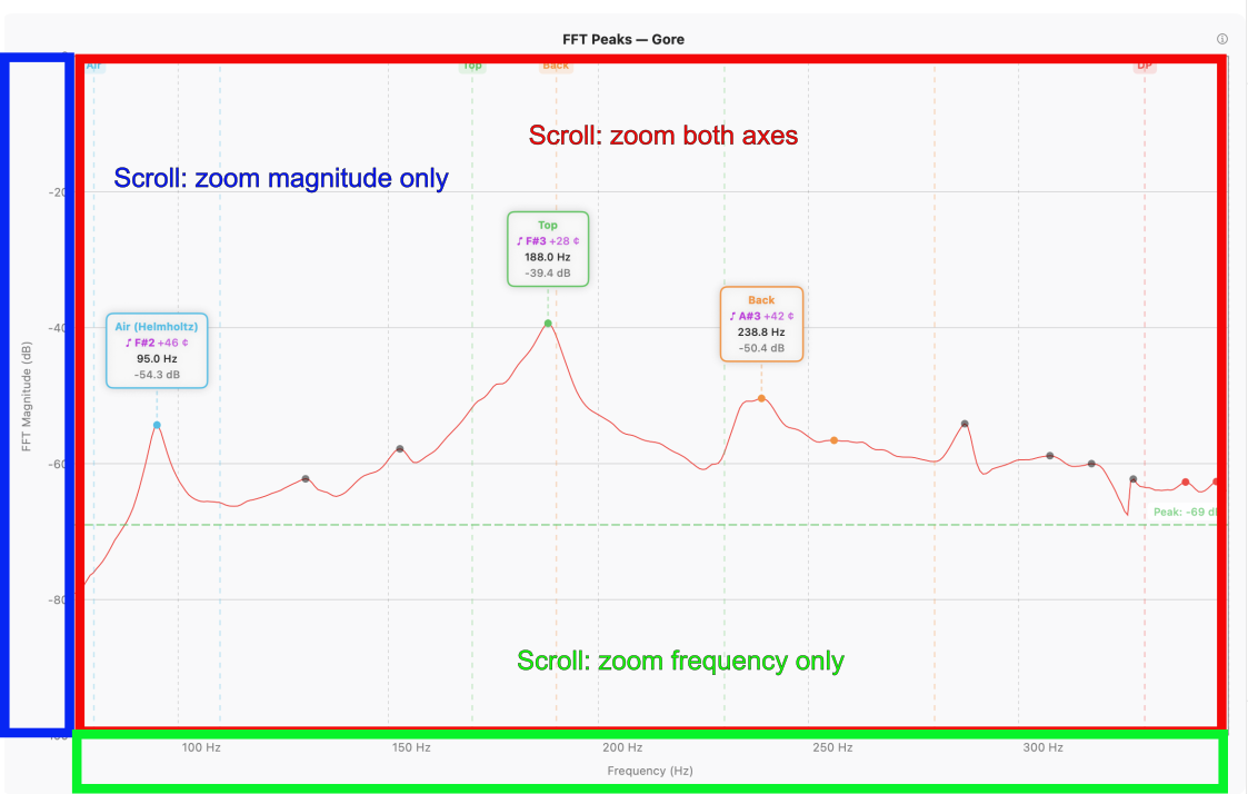
- Scroll over the plot area to zoom both axes simultaneously.
- Scroll over the frequency axis (the bottom of the chart) to zoom the frequency axis only.
- Scroll over the magnitude axis (the left edge) to zoom the magnitude axis only.
- Drag in any of the three zones to pan with the same axis-sensitivity rules.
Modifier keys augment scrolling without changing which zone you are in:
| Modifier | Scroll effect |
|---|---|
| ⇧ Shift | Pan the frequency axis |
| ⌥ Option (macOS) / Alt (Windows / Linux) | Pan the magnitude axis |
| ⌘ Command (macOS) / Ctrl (Windows / Linux) | Zoom both axes |
On a trackpad, two-finger pinch works the same as scroll-wheel zoom — over the plot area for both axes, over an axis for that axis only.
To reset the view, right-click anywhere in the chart area and choose Reset Axes from the context menu.
If you need to look the bindings up in place, the ? icon in the upper-right corner of the spectrum window opens a Zoom & Pan Controls popover that summarises all the gestures and modifier keys for the current platform.
6.4 Auto dB
Auto dB scales the magnitude axis to fit the current signal: the floor moves to just below the lowest visible value and the ceiling to just above the highest. It is the fastest way to land on a sensible magnitude range after a measurement, especially when the captured tap was much louder or quieter than the live signal that preceded it.
A button in the toolbar invokes Auto dB. The keyboard shortcut is ⌘0 on macOS; Ctrl+0 on Windows and Linux.
Use Auto dB after each measurement, or any time the spectrum clips or sits flat against the magnitude floor.
6.5 The Crosshair (iOS and iPadOS)
The crosshair is a touch-based readout for inspecting frequency and magnitude at any point on the chart.
- Tap the crosshair icon
 in the toolbar to enable it. The icon switches to
  while crosshair mode is active.
 - Touch and drag anywhere on the chart. A vertical and horizontal line follow your finger; a small readout shows the frequency (Hz) and magnitude (dB) under the crosshair.
- Tap the icon again to disable.
The crosshair is a read-only tool — it does not change the selected peaks, the spectrum, or any saved state. On desktop there is no toggle; the crosshair follows the mouse pointer continuously whenever the pointer is over the chart, showing the frequency and magnitude under the cursor in real time.
6.6 Peak Labels
Each annotated peak carries a label showing the mode name, frequency (and pitch with cents offset in guitar mode). Labels are positioned automatically to minimise overlap, but you can move any label to a position you prefer.
- Drag a label to reposition it. The new position is saved with the measurement and restored when the measurement is reloaded.
- Reset an individual label — double-tap on iOS / iPadOS; right-click and choose Reset Position on desktop.
- Reset all labels — open the … menu in the upper-right corner of the spectrum chart and choose Reset Labels on iOS / iPadOS; right-click an empty area of the chart and choose Reset Labels on desktop.
6.7 Annotation Modes
The Annotations button cycles through three states that control which peaks are labelled on the chart:
- All — every detected peak is labelled. Useful for surveying a spectrum where you have not yet decided which peaks matter.
- Selected (default) — only peaks currently selected for analysis are labelled. Matches what most luthiers want during normal use.
- None — no labels. Useful for clean export images or for reading the bare spectrum shape without distractions.
Cycle via the Annotations button, or with the keyboard shortcut
⌘** on macOS / **Ctrl+ on Windows and Linux.
Annotation mode applies to the current view only — it is not saved with the measurement, and does not affect which peaks contribute to derived values (selection does that, see §3.6).
6.8 Saving the Current View as Default
Once you have zoomed and panned to a view you want as your starting point for every new measurement, save it:
Settings → Advanced → Display Settings → Save Current View
What is saved: the frequency range (low and high Hz) and the magnitude range (low and high dB) of the current chart. The saved view becomes the target of Reset to Saved (§6.2) and of right-click → Reset Axes (§6.3) on subsequent launches.
The default view is a single global setting, not per measurement mode. If you work in plate mode and guitar mode at different ranges, pick the view that suits the work you do most often and zoom from there for the other.
Chapter 7 — Saving, Exporting, and Sharing Measurements
This chapter is a complete reference for everything you can do with a measurement after capture: store it, review it, send it elsewhere, and bring it back later.
7.1 Saving a Measurement
Press Save ![]() in the toolbar to store the
current measurement. Save is enabled whenever there is a finished
measurement on screen — a frozen single tap, a complete plate or
brace multi-phase capture, or an active comparison overlay — and
disabled when the spectrum is live or no peaks have been
identified.
in the toolbar to store the
current measurement. Save is enabled whenever there is a finished
measurement on screen — a frozen single tap, a complete plate or
brace multi-phase capture, or an active comparison overlay — and
disabled when the spectrum is live or no peaks have been
identified.
The Save sheet has two fields, both optional:
- Name — a short label identifying what you measured. For a guitar measurement this is typically the luthier's name for the instrument (a serial number, a project name, a working title). For a plate or brace it is the identifier for that specific piece (a board number, supplier code, billet label). If left blank, the date and time serve as the name.
- Notes — free text. Use it to record provenance, build-stage context, dimensions you measured by hand, or anything else you want to carry alongside the data.
What is stored depends on the type of measurement:
- Guitar / plate / brace — the spectrum (or 2–3 spectra for a plate measurement, one per phase), detected peaks and selections, settings active at capture time (subtype, plate dimensions, threshold, peak min, and so on), annotation positions, and mode overrides.
- Comparison — the constituent spectra (one per measurement that was being compared) and their colours, plus the Comparison Results table. Saving a comparison does not consume the individual measurements that were combined; they remain in the list as separate entries.
Keyboard shortcut: ⌘S on macOS; Ctrl+S on Windows and Linux.
After Save, the measurement appears at the top of the Measurements list (§7.2).
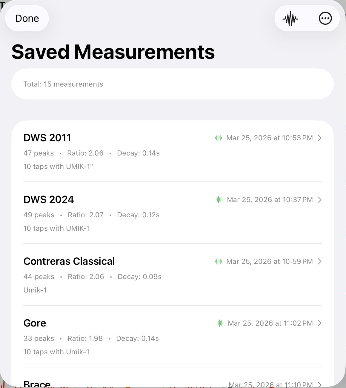
7.2 Viewing Saved Measurements
Open the Measurements list with the toolbar Measurements
button ![]() , or with ⌘L on macOS / Ctrl+L
on Windows and Linux.
, or with ⌘L on macOS / Ctrl+L
on Windows and Linux.
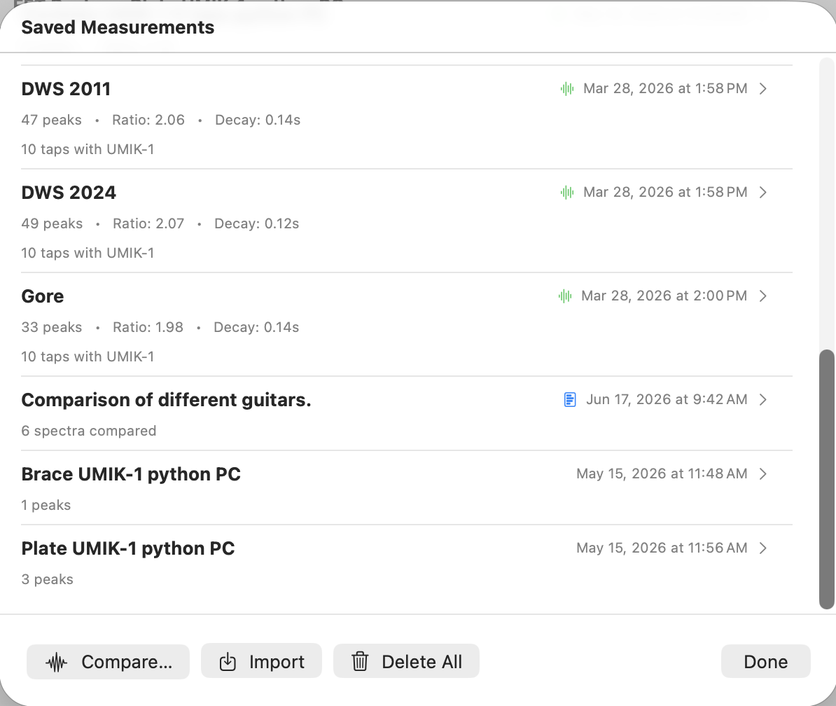
Each row carries up to three lines plus a trailing column:
- Line 1 — the name (bold; "Measurement" or "Comparison" as a fallback when no name has been set), and on the right a waveform indicator 〜 for guitar measurements that have a captured spectrum, a chart indicator for saved comparisons, the date and time of capture, and a chevron.
- Line 2 — for guitar measurements: peak count, tap-tone ratio (if available), and decay time (if available). For comparisons: "N spectra compared". For plate / brace: peak count and the headline material values.
- Line 3 — the notes you entered on Save, if any.
The list is shown in the order the measurements were saved — newest entries appear at the bottom — not sorted by date or name.
7.3 Loading a Measurement into the View
Either double-click the measurement row, or open the popup menu on the row (right-click on desktop, long-press on iOS / iPadOS) and choose Load into View.
What is restored on load:
- The frozen spectrum and its peaks
- Annotation positions
- Mode overrides
- The settings that were active at capture time
Loading a measurement replaces the analyzer's current settings — threshold, Peak Min, Taps, measurement type, and so on — with the values that were active when the measurement was captured. Your saved Settings values are untouched.
The status bar shows a "loaded settings" notice while this is in effect. The notice matters because pressing New Tap with the loaded settings active will capture using the loaded measurement's values, not the ones you had configured before. If that is not what you want, change Settings (or load a different measurement whose settings you do want) before tapping.
Loading a saved comparison restores all constituent spectra as the overlay, brings up the Comparison Results table, and switches the view into comparison mode.
7.4 Viewing Measurement Details
Open the popup menu on a measurement row (right-click on desktop, long-press on iOS / iPadOS) and choose View Details, or tap the row directly.
The detail view is read-only. It contains:
- The peak table (mode, frequency, magnitude, Q, bandwidth, pitch for guitar mode; the equivalent fields for plate / brace)
- The analysis summary (decay time and Tap Tone Ratio for guitar; E_L, E_C, specific modulus, quality rating, Gore thickness for plate / brace)
- The name and notes
For a comparison, the detail view shows the list of constituent spectra and the Air / Top / Back frequency table.
Load, Edit Name & Notes, and the export actions are reached from the popup menu on the row in the Measurements list, not from this view.
To dismiss the detail view: click the window's close button on macOS, press Close in the Python desktop build, or tap anywhere outside the dialog on iOS / iPadOS.
7.5 Editing Name and Notes
You can change a measurement's name or notes at any time after it has been saved.
Open the popup menu on the measurement row (right-click on desktop, long-press on iOS / iPadOS) and choose Edit Name & Notes. The edit sheet has the same two fields as Save. Tapping Save in the sheet commits the change immediately — there is no separate confirm step and no undo.
7.6 Exporting a Spectrum Image
Produces a PNG of the chart at display resolution. The image reflects whatever the measurement contains: a single tap is exported as one frozen spectrum with annotations, a plate measurement is exported with all of its phase spectra, and a comparison is exported as the overlay with every coloured curve, its label, and the legend.
Two ways to invoke it:
- For a measurement on screen — press the Export Spectrum button at the bottom of the Analysis Results window. Keyboard shortcut: ⌘E on macOS; Ctrl+E on Windows and Linux.
- For a saved measurement — open the popup menu on its row in the Measurements list and choose Export Spectrum.
7.7 Exporting a PDF Report
Bundles the chart, the data, and the metadata into a single shareable PDF. Like the spectrum image export, this works on any measurement; the PDF contents follow the measurement type:
- Guitar — spectrum image, peak frequency table (mode, frequency, magnitude, Q, bandwidth, pitch), and the analysis summary (decay time and Tap Tone Ratio).
- Plate / brace — spectrum image(s) for the captured phases, the peak table, and the material properties (E_L, E_C, specific modulus, radiation ratio, quality rating, and Gore thickness for plate).
- Comparison — a header listing the constituent measurements, the overlay spectrum image, and the Air / Top / Back frequency table with one column per constituent.
Every PDF carries a metadata header with the date, name, and notes.
Two ways to invoke it:
- For a measurement on screen — press the Export PDF Report button at the bottom of the Analysis Results window. Keyboard shortcut: ⇧⌘E on macOS; Ctrl+Shift+E on Windows and Linux.
- For a saved measurement — open the popup menu on its row in the Measurements list and choose Export PDF Report.
7.8 Exporting a Measurement
The native portable container is the .guitartap file — a
self-contained snapshot of a saved measurement that can be moved
to any other device and re-opened without loss.
What it contains: the peaks (with selections and mode overrides), the full spectrum data (Base64-encoded little-endian float32 arrays for frequency and magnitude), annotation positions, and the settings active at capture time. For a measurement that holds more than one spectrum — a plate measurement with its 2 or 3 phase captures, or a comparison with its constituent waveforms — every spectrum is embedded, so the file is larger but stays fully self-contained.
Which popup-menu item to use depends on platform:
- iOS / iPadOS: Export Measurement → system share sheet (AirDrop, Mail, Files, etc.).
- macOS (native build): either Export Measurement (system share sheet) or Save Measurement to Disk… (file-save dialog).
- Python build (Windows / Linux / macOS Python): Export Measurement → file-save dialog. There is no share sheet on these platforms, so the action behaves the same way as Swift macOS's Save Measurement to Disk…
The file extension is .guitartap on every platform, and the
format is interchangeable across iOS, iPadOS, macOS, Windows, and
Linux builds.
7.9 Importing a Measurement
The access path differs between platforms:
- iOS / iPadOS: open the Saved Measurements dialog, tap the
 menu in the upper-right corner, and choose Import
Measurement. (The same menu also hosts Delete All.)
The Files picker opens; select a
menu in the upper-right corner, and choose Import
Measurement. (The same menu also hosts Delete All.)
The Files picker opens; select a .guitartapto import. - Desktop (macOS native and Python builds): File → Import Measurement opens a file picker. Drag-and-drop onto the Saved Measurements window also works.
The imported measurement appears in the list regardless of its type — guitar, plate, brace, or comparison.
If the input device named in the imported file is not available on the current system, the import still succeeds and the imported data is unchanged. A warning is shown after the import completes, letting you know that further capture will use a fallback input device until the original is reconnected.
7.10 Sharing Between Devices
Anything you can export — measurements (§7.8), spectrum images (§7.6), or PDF reports (§7.7) — can be shared between devices. Which action to use depends on where the file is going.
Apple ecosystem (iOS, iPadOS, macOS native build). Use the Export Measurement, Export Spectrum, or Export PDF Report popup-menu actions. Each opens the system share sheet, from which:
- AirDrop sends directly to a nearby Apple device.
- iCloud Drive / Files stores the file to iCloud; the receiver opens it from Files on their device.
- Mail / Messages attaches the file; the recipient taps the attachment to open it.
Non-Apple devices and archival. Use Save Measurement to
Disk… (macOS popup menu) — which is the file-save path, not a
share-sheet path — to write a .guitartap directly to a folder
of your choice. On Python desktop builds (Windows, Linux, and
macOS Python) the Export Measurement action opens the same
kind of save dialog, since no system share sheet exists on
Windows or Linux. From disk the file can travel via any
cross-platform channel — Dropbox, Google Drive, email, USB drive,
network share — and the receiver imports it with §7.9. This same
disk-save path is the right choice when you simply want a
permanent file copy outside the app's library.
Cross-platform example. Export from a Windows or Linux build
with the Export Measurement action — which opens a save
dialog on those platforms — transfer the resulting .guitartap
file to an iPhone or iPad (via Files, email, Dropbox, etc.), and
import it on the receiving Apple device via §7.9. The
.guitartap format is identical on every platform, so no
conversion is needed regardless of direction.
7.11 Deleting Measurements
- Desktop: popup menu → Delete.
- iOS / iPadOS: swipe-to-delete on the row.
A confirmation prompt appears before deletion so an accidental click or swipe does not lose data. Deleting a measurement removes it and any data embedded in it; nothing else in the list is affected. Because a comparison embeds copies of its constituent spectra at save time, deleting an individual measurement that was previously combined into a comparison leaves that comparison intact, and deleting a comparison leaves its source measurements intact.
Chapter 8 — Settings Reference
The Settings sheet collects every persisted configuration the analyzer uses: audio input, measurement-type-specific inputs (mode frequency windows for guitar, dimensions for plate / brace), and the Advanced display- and analysis-tuning values.
This chapter is the reference for every field. Workflow context for the most-used ones — choosing a measurement type, tuning threshold and peak min, importing a calibration — lives in Chapter 2.
8.1 Opening Settings
- iOS / iPadOS: tap the Settings
 icon in the
main toolbar.
icon in the
main toolbar. - macOS (native build): Guitar Tap → Settings… in the application menu, or ⌘,.
- Python desktop (macOS Python): Guitar Tap → Settings… in the application menu, or ⌘,, or the Settings button in the toolbar.
- Python desktop (Windows / Linux): File → Settings…, or Ctrl+,, or the Settings button in the toolbar.
Changes apply immediately (no Apply step) and persist across launches.
8.2 Audio Input & Calibration
- Input device — picker listing the microphones available on the current system. Selecting a device makes it the active input.
- Calibration — shows the calibration file currently associated with the active input device, or "None".
- Import Calibration File — opens a file picker; accepts
.txtand.caltwo-column (frequency, dB) files. The selected file is bound to the currently active device and reloads automatically when you next select that device. - Clear All Calibrations — removes every stored calibration across all devices. Use when you want a clean baseline.
See §2.3 and §2.4 for the workflow.
8.3 Measurement Type
The Measurement Type section adapts to the type you select.
Guitar subtype — pick one of:
- Generic Guitar — broad frequency windows; recommended default.
- Acoustic Guitar — narrower windows tuned for steel-string flat-tops.
- Classical Guitar — windows for classical builds.
- Flamenco Guitar — windows for flamenco builds.
Below the subtype picker, Mode Frequency Ranges displays the windows the analyzer uses to classify air, top, back, dipole, ring, and upper modes for the chosen subtype. The display is read-only — the windows are a property of the subtype, not a user-tunable value.
Plate — the section reveals the plate inputs (described in detail in §4.3):
- Length (mm) — along the grain.
- Width (mm) — across the grain.
- Thickness (mm).
- Mass (g).
- Calculated Density — live preview computed from the four values above; sanity-check against the expected range for the wood (spruce: 0.35–0.45 g/cm³).
- Body Length (mm) and Lower Bout Width (mm) — used by the Gore target thickness calculation.
- Plate Stiffness Preset — Steel String Top (75), Steel String Back (55), Classical (50), or Custom. See §4.3 for the Custom calibration workflow.
- Measure FLC — when on, the sequence runs in three phases (L, C, FLC) instead of two (L, C).
Brace — the section reveals the brace inputs (described in detail in §5.2):
- Length (along grain) (mm).
- Width (breadth) (mm).
- Height (tap direction) (mm) — the
tdimension in the stiffness formula. The Settings panel includes a helper line below the field to flag this. - Mass (g).
- Calculated Density — same live preview as the plate section.
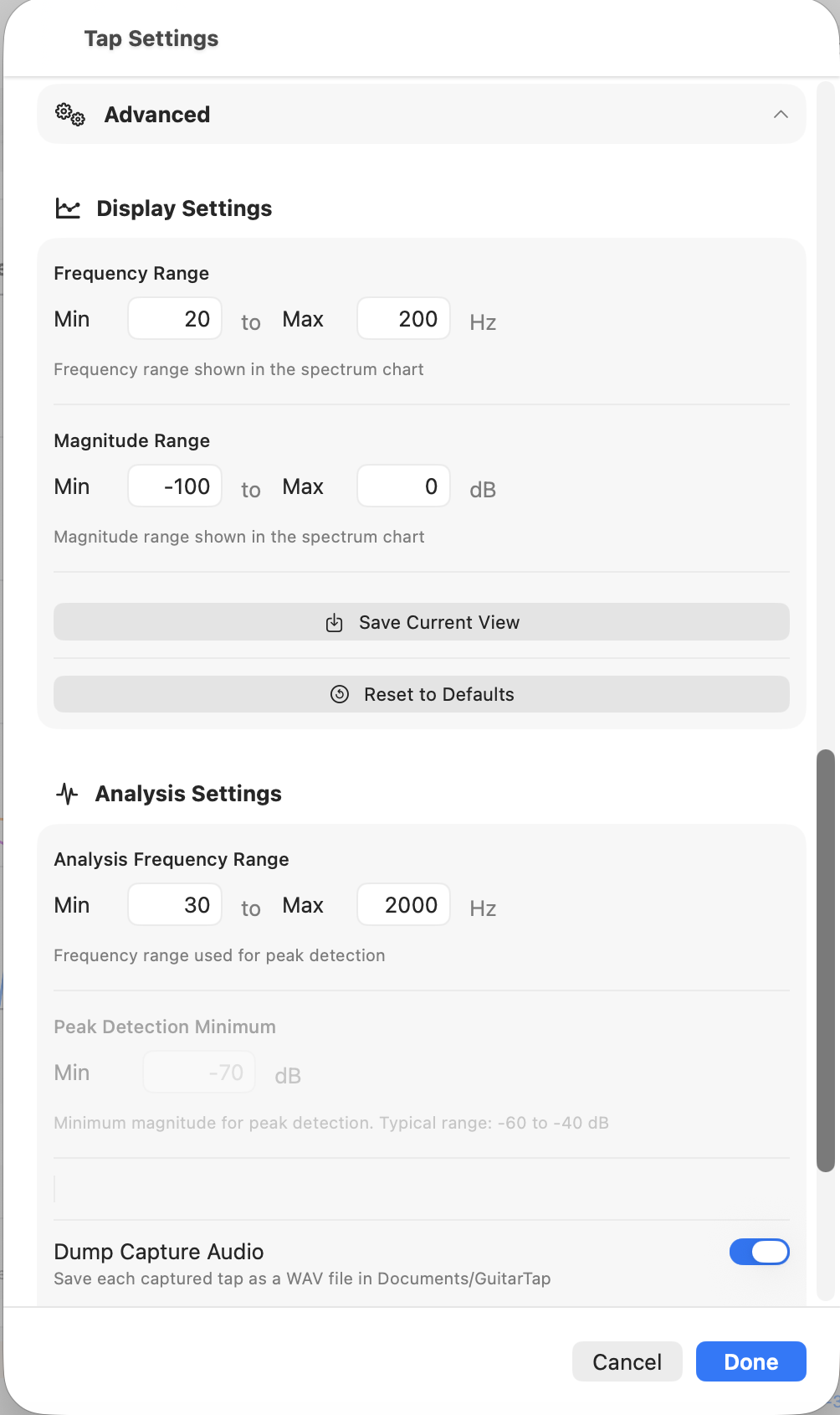
8.4 Advanced — Display Settings
Tap Advanced to reveal these.
- Frequency Range — min and max Hz shown on the spectrum chart. Defaults are wide enough to cover guitar / plate / brace ranges; narrow them when you want a closer look at a specific band.
- Magnitude Range — min and max dB shown on the chart.
- Save Current View — saves the current chart axes (frequency and magnitude ranges) as your default. Reset to Saved in the chart's … menu (§6.2) returns to this view.
- Reset to Defaults — restores the built-in starting ranges.
8.5 Advanced — Analysis Settings
- Show Unknown Modes (guitar only) — when on, peaks that do not fall within any classified mode window are still annotated on the chart. On by default; turn off to declutter a chart intended for sharing. (Cross-ref §3.1.)
- Analysis Frequency Range — min and max Hz used for peak detection. Distinct from the display frequency range above: this controls which peaks the analyzer considers, not what is shown on the chart.
- Peak Detection Minimum (guitar only) — the same Peak Min value as the toolbar slider (§2.7); the Settings field accepts a precise numeric value. Sets the minimum magnitude (dB) a peak must reach to be annotated and included in the analysis. Typical range: −60 to −40 dB. Disabled in plate / brace mode (the per-phase capture uses its own adaptive noise floor).
- Dump Capture Audio — diagnostic. When on, each captured
tap is saved as a mono 32-bit-float WAV file. Useful for
debugging; leave off in normal use. The save location is:
- macOS / Linux (native and Python builds):
~/Documents/GuitarTap/ - Windows (Python build):
%USERPROFILE%\Documents\GuitarTap\ - iOS / iPadOS: the app's sandbox Documents directory, reachable via Files → On My iPad/iPhone → Guitar Tap.
- macOS / Linux (native and Python builds):
File names are timestamped, prefixed by the originating build —
swift_<label>_<timestamp>.wav or python_<label>_<timestamp>.wav
— so dumps from cross-platform comparison runs are easy to tell
apart.
- Reset Analysis Settings — restores the analysis defaults.
8.6 About & Help
The final section of the Settings sheet carries three items:
- Version — the running build's version string.
- Copyright — the copyright line from the app's bundle metadata.
- Quick Start Guide
 — opens the in-app
Quick-Start Guide. The content matches the printable Quick-Start
PDF that ships with the app.
— opens the in-app
Quick-Start Guide. The content matches the printable Quick-Start
PDF that ships with the app. - User Manual — opens the full User Manual (this document) in the system default browser. Requires an internet connection; the manual is hosted at dolcesfogato.com.
Chapter 9 — Controls Reference
A scannable reference for every button, control, and gesture. For the workflows that exercise them, see Chapters 3–7. For the chart-interaction details, see Chapter 6.
9.1 Toolbar — iOS iPhone (Portrait)
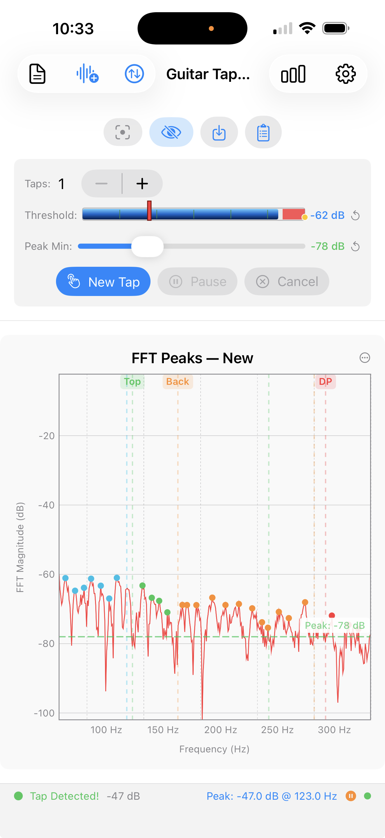
Vertical layout with three stacked control rows above the chart.
Top — navigation toolbar:
- Leading (left): Results
 ,
Play File
,
Play File  ,
Auto dB
,
Auto dB  .
. - Trailing (right): Metrics
 ,
Settings .
,
Settings .
Middle — secondary icon row (just below the toolbar):
- Crosshair ,
Annotations
 ,
Save
,
Save  ,
Measurements
,
Measurements  .
.
Bottom — Tap Controls panel (§9.6):
Taps stepper, Threshold slider, Peak Min slider, and the action buttons New Tap / Pause-Resume-Accept / Cancel-Redo.
9.2 Toolbar — iOS iPhone (Landscape)
Horizontal split layout with the Tap Controls in a vertical panel on the left and the spectrum chart filling the right side. The navigation toolbar runs across the top of the screen.
- Leading: Results ,
Play File ,
Auto dB ,
Crosshair ,
Annotations .
- Trailing: Save ,
Measurements ,
Metrics ,
Settings ,
Help .
The Tap Controls panel scrolls vertically when there is not enough height to show every control at once.
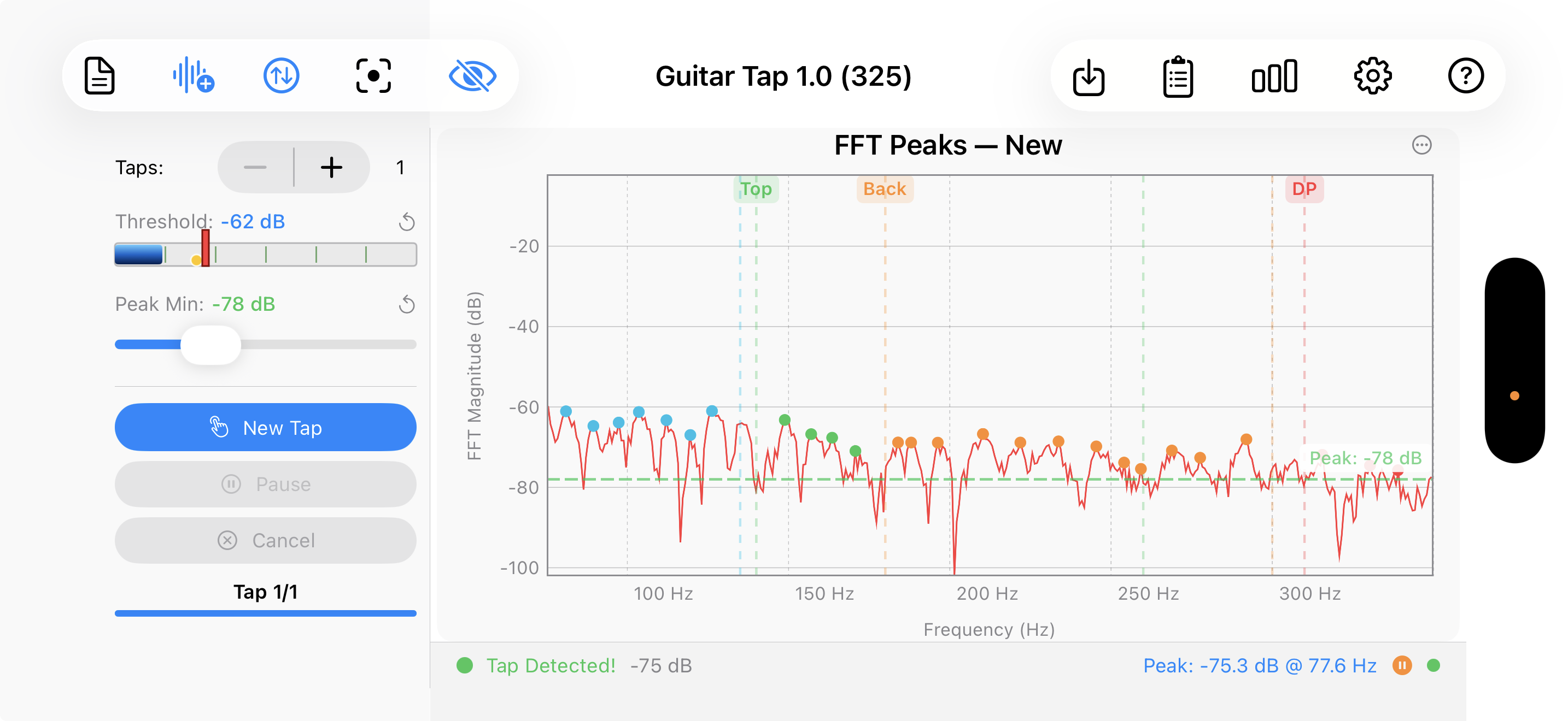
9.3 Toolbar — iOS iPad
iPad uses a single layout in both portrait and landscape (the
horizontal size class is .regular in either orientation, so the
same inline three-pane arrangement applies). The Analysis Results
panel is shown inline alongside the chart — like the desktop
layout — so the toolbar does not include a Results button.
- Leading: Play File ,
Auto dB ,
Crosshair ,
Annotations .
- Trailing: Save ,
Measurements ,
Metrics ,
Settings ,
Help .
The full Tap Controls panel is visible above the chart in both orientations.
9.4 Menu Bar — Desktop
Both the Swift native macOS build and the Python desktop build (Windows, Linux, macOS Python) expose the same operations through a menu bar. The placement and shortcuts differ per platform following the host OS conventions.
Application menu (macOS — both native and Python; on Windows and Linux these items move into the File and Help menus per the notes below):
| Item | macOS shortcut |
|---|---|
| About Guitar Tap | (system default) |
| Settings… | ⌘, |
| Quit Guitar Tap | ⌘Q |
File menu:
| Item | macOS shortcut | Windows / Linux shortcut |
|---|---|---|
| Close (macOS only) | ⌘W | — |
| Play Audio File… | ⌘⌥O | Ctrl+Alt+O |
| Save Measurement… | ⌘S | Ctrl+S |
| Export Spectrum Image… | ⌘E | Ctrl+E |
| Export PDF Report… | ⇧⌘E | Ctrl+Shift+E |
| Settings… (Win / Linux Python only) | — | Ctrl+, |
| Exit / Quit (Win / Linux Python only) | — | (system default) |
View menu:
| Item | macOS shortcut | Windows / Linux shortcut |
|---|---|---|
| Auto dB | ⌘0 | Ctrl+0 |
| Cycle Annotations | ⌘` | Ctrl+` |
| Show Metrics | ⌘M | Ctrl+M |
| Show Measurements | ⌘L | Ctrl+L |
Help menu:
| Item | macOS shortcut | Windows / Linux shortcut |
|---|---|---|
| Quick Start Guide | ⌘? | F1 |
| User Manual | — | — |
| About Guitar Tap… (Win / Linux Python only) | — | (no default) |
9.5 Individual Controls
Each entry: icon, name, what it does, and any platform notes. Keyboard shortcuts are given in macOS form first followed by Windows / Linux where they differ.
New Tap ![]() — Arms the tap detector, clears the
frozen spectrum, and returns to the live view. Also exits
comparison mode when a comparison is active. Always enabled
unless detection is unavailable.
— Arms the tap detector, clears the
frozen spectrum, and returns to the live view. Also exits
comparison mode when a comparison is active. Always enabled
unless detection is unavailable.
Play File ![]() — Opens a
file picker; the selected audio file is fed through the analysis
pipeline as if it were live microphone input. Useful for analyzing
captured WAVs or running the analyzer against a reference
recording. The icon tints orange while a file is playing. Also
reached from the desktop menu bar (File → Play Audio File…,
⌘⌥O macOS / Ctrl+Alt+O Windows / Linux).
— Opens a
file picker; the selected audio file is fed through the analysis
pipeline as if it were live microphone input. Useful for analyzing
captured WAVs or running the analyzer against a reference
recording. The icon tints orange while a file is playing. Also
reached from the desktop menu bar (File → Play Audio File…,
⌘⌥O macOS / Ctrl+Alt+O Windows / Linux).
Pause ![]() /
Resume
/
Resume ![]() /
Accept
/
Accept ![]() — A
single button whose label and icon change with state.
Pause suspends tap detection while keeping the spectrum live
— use it to tune Threshold and Peak Min freely (§2.6, §2.7).
Resume re-arms detection. Accept (green) replaces the
pair during plate / brace review phases (§4.5) and locks in the
current phase result before advancing.
— A
single button whose label and icon change with state.
Pause suspends tap detection while keeping the spectrum live
— use it to tune Threshold and Peak Min freely (§2.6, §2.7).
Resume re-arms detection. Accept (green) replaces the
pair during plate / brace review phases (§4.5) and locks in the
current phase result before advancing.
Cancel ![]() /
Redo
/
Redo ![]() —
A single button whose label and icon change with state.
Cancel discards the active sequence and returns to the live
view. During a plate / brace review phase it becomes Redo L,
Redo C, or Redo FLC (orange) and re-arms detection for
that phase only (§4.5).
—
A single button whose label and icon change with state.
Cancel discards the active sequence and returns to the live
view. During a plate / brace review phase it becomes Redo L,
Redo C, or Redo FLC (orange) and re-arms detection for
that phase only (§4.5).
Results ![]() (iPhone only) — Opens the
Analysis Results sheet.
(iPhone only) — Opens the
Analysis Results sheet.
Auto dB ![]() — Scales
the magnitude axis to fit the current signal (§6.4). Shortcut:
⌘0 / Ctrl+0.
— Scales
the magnitude axis to fit the current signal (§6.4). Shortcut:
⌘0 / Ctrl+0.
Annotations ![]() /
/
![]() /
/
![]() —
Cycles through the annotation display modes: All → Selected →
None → All … (§6.7). The icon shows which state is currently
active. Shortcut: ⌘` / Ctrl+`.
—
Cycles through the annotation display modes: All → Selected →
None → All … (§6.7). The icon shows which state is currently
active. Shortcut: ⌘` / Ctrl+`.
Save ![]() —
Opens the Save Measurement sheet (§7.1). Enabled whenever there
is a finished measurement on screen — single tap, plate / brace
multi-phase capture, or active comparison overlay. Shortcut:
⌘S / Ctrl+S.
—
Opens the Save Measurement sheet (§7.1). Enabled whenever there
is a finished measurement on screen — single tap, plate / brace
multi-phase capture, or active comparison overlay. Shortcut:
⌘S / Ctrl+S.
Measurements ![]() —
Opens or closes the Measurements list (§7.2). Shortcut: ⌘L /
Ctrl+L.
—
Opens or closes the Measurements list (§7.2). Shortcut: ⌘L /
Ctrl+L.
Metrics ![]() — Opens or closes the FFT
Diagnostics panel (frame rate, FFT size, input level, and so
on). Shortcut: ⌘M / Ctrl+M.
— Opens or closes the FFT
Diagnostics panel (frame rate, FFT size, input level, and so
on). Shortcut: ⌘M / Ctrl+M.
Crosshair ![]() /
/
![]() (iOS /
iPadOS only) — Toggles the touch-readout crosshair (§6.5). On
desktop there is no toggle; the crosshair follows the mouse
pointer whenever the pointer is over the chart, showing the
frequency and magnitude under the cursor in real time.
(iOS /
iPadOS only) — Toggles the touch-readout crosshair (§6.5). On
desktop there is no toggle; the crosshair follows the mouse
pointer whenever the pointer is over the chart, showing the
frequency and magnitude under the cursor in real time.
Chart Options ![]() (iOS / iPadOS
only) — Opens the Chart Options sheet from the upper-right
corner of the spectrum chart. Hosts the Reset to Saved and Reset
to Defaults groups, plus Reset Labels when there are dragged
labels to reset (§6.2, §6.6). On desktop the same actions are
reached by right-clicking the chart.
(iOS / iPadOS
only) — Opens the Chart Options sheet from the upper-right
corner of the spectrum chart. Hosts the Reset to Saved and Reset
to Defaults groups, plus Reset Labels when there are dragged
labels to reset (§6.2, §6.6). On desktop the same actions are
reached by right-clicking the chart.
Zoom & Pan Help ![]() (desktop only) — Shows a
summary popover of the scroll, modifier-key, and trackpad
gestures for axis zoom and pan (§6.3).
(desktop only) — Shows a
summary popover of the scroll, modifier-key, and trackpad
gestures for axis zoom and pan (§6.3).
Settings ![]() — Opens the Settings sheet
(Chapter 8). Shortcut: ⌘, / Ctrl+,.
— Opens the Settings sheet
(Chapter 8). Shortcut: ⌘, / Ctrl+,.
Help ![]() — Opens a small menu with
two items: Quick Start Guide (the in-app help content; also
reachable directly via ⌘? on macOS or F1 on Windows /
Linux) and User Manual (opens the published manual in the
system browser). On iOS and iPadOS the menu lives behind the
toolbar ? button; on desktop the same two items appear in
the Help menu bar.
— Opens a small menu with
two items: Quick Start Guide (the in-app help content; also
reachable directly via ⌘? on macOS or F1 on Windows /
Linux) and User Manual (opens the published manual in the
system browser). On iOS and iPadOS the menu lives behind the
toolbar ? button; on desktop the same two items appear in
the Help menu bar.
9.6 Tap Controls
The Tap Controls panel groups the per-measurement settings and action buttons. Its placement varies by platform — see §9.1 (iPhone portrait), §9.2 (iPhone landscape), §9.3 (iPad), and §9.4 (desktop) for where it sits on each layout. The contents themselves are the same everywhere:
-
Taps stepper (1 – 10) — number of taps to capture in each guitar-mode sequence, or per phase in plate / brace mode (e.g. 3 means three taps for Longitudinal, three for Cross-grain, and three for FLC if enabled). Disabled while a sequence is in progress and during comparison mode.
-
Threshold slider — signal level (dB) that triggers tap detection (§2.6). The current value is shown next to the slider; the reset arrow restores the factory default. Range: −80 dB to −20 dB. Disabled during comparison mode.
-
Peak Min slider — minimum spectrum magnitude (dB) at which a peak is annotated on the chart and included in guitar-mode analysis (§2.7, §8.5). The current value is shown next to the slider; the reset arrow restores the factory default. Range: −100 dB to −20 dB. In plate / brace mode the slider affects only what is drawn on the chart — the selected peak for each phase comes from the capture algorithm and is not changed by Peak Min. Disabled during comparison mode and during plate / brace measurements.
9.7 Status Bar
A thin status bar runs below the spectrum chart on every platform and orientation. It is a read-only feedback area that reflects the current state of the analyzer; the contents change with state.
Normal tap-detection (default). Left to right:
- A circle indicator — green when a tap has been captured (label: Tap Detected!), grey while waiting (Waiting for tap…).
- The current input level in dB.
- During a multi-tap guitar sequence or a plate / brace sequence: a counter such as Tap 2/3 or Phase 1/2 · Tap 1/3, plus a thin progress bar.
- Peak: X.X dB @ Y.Y Hz — the loudest spectrum bin in the current view, shown on the right side.
- A pause-fill glyph when the spectrum has frozen on a completed measurement.
- A small circle indicating audio-engine state — green for running, red for stopped.
Loaded-settings warning. After a saved measurement is loaded (see §7.3) the bar shows an orange triangle and the message Loaded settings — Threshold: X dB · Taps: N. The notice remains visible until you change Settings or start a fresh capture.
Comparison mode. A waveform glyph and a one-line description of the comparison — Comparing N measurements for a saved comparison, or Tap comparison — N taps + averaged for the multi-tap comparison view — plus a hint about how to exit the mode (press Taps or New Tap).
The iPhone layout uses a single-line condensed version of this bar; the iPad and desktop layouts use a slightly taller version that stacks the warning above the tap-state row when both apply at once.
9.8 Spectrum Chart Interactions
See Chapter 6 for a complete reference covering live and frozen state, zoom / pan gestures and shortcuts, the ? popover, the crosshair, peak-label dragging and reset, and the Annotation modes cycle.
Chapter 10 — Tips, Technique, and Troubleshooting
Practical advice for tighter results, plus a table of common problems and their fixes.
10.1 Tap Technique
The cleanest impulse comes from a small bouncy ball on the end of a stick. Short contact time, clean impulse, low operator variability, and reproducible day to day. Works for all three modes (guitar, plate, brace).
A firm knuckle or fingertip rap is the day-to-day alternative for guitar-body surveys and works well there. It is less ideal for plate and brace measurements because contact time varies more.
Contact time matters. A long slow push excites fewer overtones and muddies the spectrum; the shorter the contact, the better the high-frequency content. If the spectrum looks smeared-out around the peaks you care about, suspect contact time before suspecting the mic or the room.
Tap location:
- Guitar body — on the bridge centered, on each wing of the bridge, below the bridge centered, on each side. The decision comes from experience and which node excitation is desired.
- Plate or brace — centre of the face. Off-centre taps bias the result; the centre is at the antinode of every mode the measurement is designed to capture.
Force. The tap does not have to be loud — it just has to clear Threshold (§2.6). An unnecessarily hard tap is more likely to trigger double-detection or saturate the input than a deliberate, medium tap.
10.2 Consistent Microphone Position
The wood's resonant frequencies are fixed; only the magnitude the microphone sees depends on where the mic is sitting. Position therefore matters for any comparison you make over time — across build stages, across thinning passes, across instruments.
Mark the position with a piece of tape or a chalk line on the bench. When you come back tomorrow, set up against the same mark.
Distance: 5–15 cm is a useful range. Closer than 5 cm risks off-axis rejection from a directional mic; further than ~20 cm gives away signal-to-noise without much benefit.
10.3 Dealing with Background Noise
The Threshold slider is the first line of defence. Move it higher (closer to 0 dB) to reject ambient noise; lower (more negative) to catch quieter taps. The goal is to put Threshold comfortably above the noise floor and comfortably below your tap peak.
The detector also applies a 3 dB hysteresis margin: after a tap fires, the signal must drop 3 dB below Threshold before the detector re-arms. This prevents the ring-out tail from re-triggering as a second tap. The 3 dB value is fixed and is appropriate for typical rooms.
Practical target. Keep your noise floor at least 10 dB below Threshold; if it is closer, false triggers become likely.
Pausing to measure the noise floor. Press Pause (§2.6), leave the analyzer running, and watch the live spectrum for a few seconds. Sustained noise peaks tell you where the noise floor sits; pick Threshold a comfortable margin above them.
Worst offenders. HVAC fans, refrigerator compressors, traffic, and computer fans. Plate and brace measurements that need to compare cleanly across days are worth either silencing or moving away from these sources.
10.4 Decoupling the Top from the Air Mode
A normal tap of the guitar body excites the air (Helmholtz) mode and the top mode together, and the two are coupled — the displayed top frequency is pulled away from the wood's true value by the coupling.
To read the top resonance without that bias, block the air cavity before tapping: stuff a rag, foam, or other soft fill into the sound hole so air cannot pump in and out. With the cavity blocked the Helmholtz resonance disappears from the spectrum, and the top peak shifts to the position it would have without air coupling.
Tap, capture, and read the top frequency. Remove the fill before returning to normal use.
10.5 Ring-Out and Decay Time
Ring-out (decay time) is the time, in seconds, for the tap's amplitude envelope to fall to 1/e (~37%) of its peak. It is a direct read on structural damping.
- Higher decay time → lower damping → more sustain.
- Lower decay time → more damping → energy is being absorbed faster.
Typical soundboard ranges:
- > 1.5 s — excellent.
- 1.0–1.5 s — good.
- < 0.8 s — worth investigating; may indicate over-drying or excessive internal friction.
Before-and-after. A top plate before bracing typically has a higher decay time than after bracing. Measuring at each stage quantifies how much the bracing is damping the resonance — a useful data point for tracking your own bracing pattern's behaviour over multiple builds.
Decay time is computed from the tap capture. In a multi-tap sequence the averaged-capture decay is reported.
10.6 Multi-Tap Averaging Strategy
The right tap count depends on what you are measuring:
- Guitar body survey — 1–3 taps. The body resonances are stable; averaging mainly reduces the impact of an occasional noisy or missed tap.
- Plate or brace material measurement — 3–5 taps. Averaging reduces variance from finger noise and small position differences, which matters for the absolute E_L value.
- FLC tap (plate mode) — 1–3 taps. The FLC resonance is weaker, so position consistency matters more than averaging. Tapping the FLC repeatedly with imperfect positioning can increase variance rather than reduce it.
When averaging helps least. Very quiet room, experienced tapper, firm bouncy-ball implement: single-tap is usually sufficient.
Sanity check. For a new piece of stock or a new technique, take a single tap and a 5-tap average of the same blank and compare the frequencies. If they agree to within 1 Hz you can trust single-tap measurements for that piece going forward.
Pause within a sequence. Press Pause after any captured tap to reposition your hand or settle the room; Resume re-arms the detector for the next tap.
10.7 Common Problems
| Problem | Likely cause | Fix |
|---|---|---|
| No tap detected | Threshold too high | Lower the Threshold slider (§2.6). |
| False detections | Threshold too low, or noisy room | Raise Threshold; verify the noise floor with Pause (§10.3). |
| Peaks missing on the chart | Peak Min too high | Lower the Peak Min slider (§2.7). |
| Unknown peaks everywhere | Analysis range too wide for the measurement | Narrow Analysis Frequency Range in Settings → Advanced → Analysis Settings (§8.5). |
| Spectrum doesn't update | Microphone permission not granted | iOS / iPadOS: Settings → Guitar Tap → Microphone. macOS: System Settings → Privacy & Security → Microphone. Windows: Settings → Privacy & Security → Microphone. Linux: check pavucontrol (§2.2). |
| Plate calculation missing | Dimensions not entered | Settings → Measurement Type → Plate; fill in Length / Width / Thickness / Mass (§4.3, §8.3). |
| Gore thickness shows "G_LC assumed 0" | FLC tap not captured | Enable Measure FLC in Settings and re-run the plate sequence (§4.8). |
| Analysis Results panel not visible (desktop) | Window too narrow | Widen the window. |
| Plate / brace stuck waiting for next phase | Accept not pressed | Look for Accept (green checkmark) in the tap controls — it replaces Pause during the review phase (§4.5). |
| Plate / brace: need to redo a phase already accepted | Phase locked in | Press New Tap to restart the whole sequence. Per-phase redo is only available before that phase is accepted. |
| Compare button does not appear | Fewer than 2, more than 5, or a plate / brace measurement is in the selection | Select 2–5 guitar measurements only (§3.9). |
| Threshold / Taps differ from your Settings after loading a measurement | Loaded measurement's settings are active | The status bar shows a Loaded settings notice (§7.3 and §9.7). Change Settings, or press New Tap to start fresh with your own values. |
| Imported file: input device warning after import | Mic named in the file isn't on this system | The import succeeded; a fallback device is in use. Reconnect the original mic, or pick a current one in Settings → Audio Input (§7.9). |
Chapter 11 — Glossary
Air (Helmholtz) mode — The resonance of the air cavity inside the instrument body, excited by the motion of air through the sound hole. Also called the Helmholtz resonance.
Bandwidth (−3 dB) — The width of a spectral peak measured at 3 dB below its maximum. Narrower bandwidth (higher Q) indicates lower damping.
Cross/Long ratio — The ratio of cross-grain Young's modulus to longitudinal Young's modulus (E_C / E_L). For spruce, typically 0.04–0.08.
Decay time — The time (in seconds) for a tap response to decay to 1/e of its peak amplitude. A measure of structural damping; higher values indicate lower damping.
Dipole mode — A bending mode of the guitar top plate where the upper and lower bouts move in opposite phase.
E_C (Young's modulus, cross-grain) — Stiffness of the wood measured perpendicular to the grain direction (radial or tangential). Expressed in GPa.
E_L (Young's modulus, longitudinal) — Stiffness of the wood measured along the grain direction. Expressed in GPa. The primary stiffness parameter for tonewood selection.
FFT (Fast Fourier Transform) — The algorithm used to convert the time-domain microphone signal into the frequency-domain spectrum displayed by the app.
FLC tap — A third tap measurement (Free-Length-Cross) used in Plate mode to estimate the shear modulus G_LC, which feeds the Gore target thickness calculation. Optional — when omitted the Gore thickness is reported with the message "G_LC assumed 0" and carries an over-estimate of roughly 5–7% (§4.8).
Free-free beam — A beam suspended at its bending-mode nodal points (22% from each end), leaving it free to vibrate without damping at the supports. The standard suspension assumption for Plate and Brace material measurements. In practice a single hold at one of the two nodal points is sufficient — see §4.4.
Free-Length-Cross (FLC) mode — The torsional mode excited by the FLC tap; its frequency feeds the shear-modulus calculation. See FLC tap.
G_LC (shear modulus) — The shear modulus of the plate, derived from the FLC tap frequency. Required by the full Gore target thickness formula; substituted with zero when FLC is not measured.
Gore target thickness — The recommended final thickness for a guitar top or back plate, calculated from the plate dimensions, Young's moduli, and a stiffness target, following the method described by Trevor Gore.
Q factor — Quality factor; the ratio of a resonant peak's centre frequency to its −3 dB bandwidth. Q = f₀ / Δf. Higher Q indicates lower damping.
Radiation ratio (R) — A figure of merit for tonewood; R = c_L / √ρ = √(E_L/ρ³). Higher values indicate a lighter, stiffer wood that radiates sound more efficiently.
Ring mode — A symmetric bending mode of the guitar top plate involving the rim of the lower bout.
Specific modulus (E/ρ) — Young's modulus divided by density. Also written as c² (where c is the speed of sound in the material). A key predictor of tap tone quality.
Speed of sound (c) — The speed at which a longitudinal stress wave travels through the wood: c_L = √(E_L / ρ). Expressed in m/s.
Tap Tone Ratio — The ratio of the top mode frequency to the air mode frequency (f_top / f_air). Typical range for a well-voiced guitar: 1.8–2.4.
Top / Back mode — The fundamental bending mode of the guitar top plate or back plate, respectively; often the strongest peak in a guitar tap spectrum.
Unknown mode — A detected spectral peak that does not fall within any defined frequency window for the selected guitar subtype. Shown on the chart by default; can be hidden with Settings → Advanced → Analysis Settings → Show Unknown Modes (§3.1, §8.5). An Unknown peak can be re-identified by tapping its row in the Analysis Results panel and assigning a standard mode (Air, Top, Back, Dipole, Ring, Upper Modes) or a custom label (§3.7).
Upper modes — Resonant modes above the main top and back modes; their significance increases with frequency and build stage.
Appendix A — Keyboard Shortcuts
Desktop keyboard shortcuts for every action with one assigned in Guitar Tap, grouped by the menu where the action appears. The same shortcuts are listed in §9.4 alongside the menu items themselves; this appendix is the lookup table.
The Swift native macOS build and the Python desktop build (Windows, Linux, macOS Python) follow the host OS conventions — ⌘ shortcuts on macOS, Ctrl shortcuts on Windows and Linux.
Application menu
| Action | macOS | Windows / Linux |
|---|---|---|
| Settings | ⌘, | Ctrl+, |
| Quit | ⌘Q | (system default) |
File menu
| Action | macOS | Windows / Linux |
|---|---|---|
| Close | ⌘W | — |
| Play Audio File | ⌘⌥O | Ctrl+Alt+O |
| Save Measurement | ⌘S | Ctrl+S |
| Export Spectrum Image | ⌘E | Ctrl+E |
| Export PDF Report | ⇧⌘E | Ctrl+Shift+E |
View menu
| Action | macOS | Windows / Linux |
|---|---|---|
| Auto dB | ⌘0 | Ctrl+0 |
| Cycle Annotations | ⌘` | Ctrl+` |
| Show Metrics | ⌘M | Ctrl+M |
| Show Measurements | ⌘L | Ctrl+L |
Help menu
| Action | macOS | Windows / Linux |
|---|---|---|
| Quick Start Guide | ⌘? | F1 |
iOS and iPadOS do not expose menu items or keyboard shortcuts in Guitar Tap; everything on those platforms is reached through the toolbar (Chapter 9) or the popup menu in the Measurements list (§7.2).
Appendix B — File Formats
Measurement files (`.guitartap`)
The native portable measurement container. UTF-8 JSON, self-contained, and identical across every platform Guitar Tap runs on (iOS, iPadOS, macOS native, and the Python build on Windows / Linux / macOS Python). A file written on any platform opens on any other without conversion. The export and import workflows are documented in §7.8 and §7.9.
The remainder of this section is a structural reference for
anyone parsing or generating .guitartap files outside the app.
File-level structure
The file is pretty-printed JSON. The top-level value is an array containing exactly one measurement object — the array wrapping is part of the format and parsers must accept it even when only one measurement is present.
[
  {
    "id": "…",
    "timestamp": "…",
    ...
  }
]
Dates are ISO-8601 strings (YYYY-MM-DDTHH:MM:SSZ). UUIDs are
RFC 4122 strings. Numbers are JSON numbers (single-precision
floats are encoded as decimal; per-spectrum arrays use the
compact binary encoding below).
Measurement object
Required fields:
| Field | Type | Notes |
|---|---|---|
id |
UUID | Stable identifier. |
timestamp |
ISO-8601 | When the measurement was saved. |
peaks |
array of Peak | All detected peaks (empty for a saved comparison). |
Optional fields — populated depending on measurement type and on what the user did at save time:
| Field | Type | Notes |
|---|---|---|
measurementName |
string | User-entered name (§7.1). |
notes |
string | User notes. |
decayTime |
float | Seconds; guitar only. |
spectrumSnapshot |
SpectrumSnapshot | Averaged guitar spectrum. |
longitudinalSnapshot, crossSnapshot, flcSnapshot |
SpectrumSnapshot | Plate / brace per-phase spectra. |
selectedLongitudinalPeakID, selectedCrossPeakID, selectedFlcPeakID |
UUID | The peak chosen as L / C / FLC. |
selectedPeakIDs |
array of UUID | Currently-selected peaks (guitar). |
selectedPeakFrequencies |
array of float | Frequencies (Hz) parallel to the IDs, used to re-match after a Peak Min change generates new UUIDs. |
peakAnnotationOffsets |
object | Map of peak UUID → { "x": <freq Hz>, "y": <magnitude dB> }. Custom label positions. |
annotationVisibilityMode |
string | Enum: all / selected / none. |
tapDetectionThreshold |
float | Threshold (dB) at save time. |
numberOfTaps |
int | Taps stepper value at save time. |
peakMinThreshold |
float | Peak Min (dB) at save time. |
peakModeOverrides |
object | Map of peak UUID → user-assigned mode label. |
microphoneName, microphoneUID |
string | Input device provenance. |
calibrationName |
string | Active calibration profile, if any. |
comparisonEntries |
array of ComparisonEntry | Present only for saved comparisons. |
tapEntries |
array of TapEntry | Per-tap data for multi-tap guitar. |
measurementType, guitarType |
string | Convenience copies for external consumers; mirror spectrumSnapshot fields. |
SpectrumSnapshot
Required fields:
| Field | Type | Notes |
|---|---|---|
frequenciesData |
Base64 string | See "Spectrum data encoding" below. |
magnitudesData |
Base64 string | Same length as frequenciesData. |
minFreq, maxFreq |
float | Chart frequency range (Hz). |
minDB, maxDB |
float | Chart magnitude range (dB). |
isLogarithmic |
bool | Axis scale. |
Optional measurement-type fields:
| Field | Type | Notes |
|---|---|---|
showUnknownModes |
bool | Mirrors the Settings toggle. |
guitarType |
string | generic / acoustic / classical / flamenco. |
measurementType |
string | generic / acoustic / classical / flamenco / plate / brace. |
plateLength, plateWidth, plateThickness, plateMass |
float | Plate dimensions in mm / g. |
guitarBodyLength, guitarBodyWidth |
float | Body inputs for Gore thickness (mm). |
plateStiffnessPreset |
string | steelStringTop / steelStringBack / classical / custom. |
customPlateStiffness |
float | Value when preset is custom. |
measureFlc |
bool | Whether the FLC phase was captured. |
braceLength, braceWidth, braceThickness, braceMass |
float | Brace dimensions in mm / g. |
Spectrum data encoding
frequenciesData and magnitudesData are Base64-encoded byte
strings. After Base64 decoding the bytes are a contiguous
little-endian IEEE-754 single-precision (float32) array — 4
bytes per value, length implicit (byteCount / 4). The two
arrays are the same length and are parallel: element i of
magnitudesData is the magnitude (dB) at the frequency (Hz)
given by element i of frequenciesData.
Reference decoder (Python):
import base64, struct
b = base64.b64decode(snapshot["frequenciesData"])
freqs = list(struct.unpack(f"<{len(b)//4}f", b))
Peak
| Field | Type | Notes |
|---|---|---|
id |
UUID | Stable identifier within the measurement. |
frequency |
float | Hz. |
magnitude |
float | dB. |
quality |
float | Q factor. |
bandwidth |
float | −3 dB bandwidth, Hz. |
timestamp |
ISO-8601 | When the peak was detected. |
pitchNote |
string | Nearest equal-temperament note, e.g. "D4". |
pitchCents |
float | Cents offset from pitchNote. |
pitchFrequency |
float | Frequency of pitchNote in Hz. |
ComparisonEntry (when `comparisonEntries` is present)
| Field | Type | Notes |
|---|---|---|
id |
UUID | Identifier for the overlay entry. |
label |
string | Display label shown in the legend. |
colorComponents |
array of 4 floats | RGBA, each 0.0 – 1.0. |
snapshot |
SpectrumSnapshot | Full spectrum data for this overlay curve. |
peaks |
array of Peak | Peaks for this overlay's source measurement. |
guitarType |
string | For mode classification. |
sourceMeasurementID |
UUID | The measurement this entry was created from, if known. |
When comparisonEntries is non-null the measurement is a saved
comparison: the top-level peaks, spectrumSnapshot,
decayTime, and similar fields are not meaningful and should
not be read.
TapEntry (when `tapEntries` is present)
Present only for guitar multi-tap measurements (numberOfTaps > 1).
Each entry preserves the raw spectrum and peaks for one tap so
the multi-tap comparison view can be reconstructed:
| Field | Type | Notes |
|---|---|---|
id |
UUID | |
tapIndex |
int | 1-based display index. |
snapshot |
SpectrumSnapshot | Raw single-tap spectrum. |
peaks |
array of Peak | Peaks detected in this single tap. |
selectedPeakIDs |
array of UUID | Auto-selected modes for this tap. |
Calibration files (`.txt` / `.cal`)
Frequency-response compensation data for a measurement
microphone. Plain text; each data line carries a frequency and a
magnitude correction, separated by tab, space, or comma.
Either of the two common vendor formats works directly — UMIK-1
.txt files and Room EQ Wizard .cal files are both accepted:
"Sens Factor =-1.2 dB, SERNO 7123456"
"Frequency (Hz)   Magnitude (dB)"
20.0      -1.2
50.0      -0.4
100.0      0.0
...
20000.0   -3.1
Header and comment lines begin with " (UMIK-1) or * (REW)
and are skipped. Only frequencies in the range 1 Hz to
24,000 Hz are used; values outside that range are ignored.
The app applies the inverse of this curve to the incoming spectrum so that the displayed result reflects the wood, not the microphone. Calibrations bind per-input-device — see §2.4 for the import workflow.
Exported formats
The export actions described in §7.6 – §7.8 produce these file types:
| Action | Extension | Contents |
|---|---|---|
| Export Measurement / Save Measurement to Disk | .guitartap |
Full measurement — peaks, spectrum data, settings, metadata (see above). |
| Export Spectrum Image | .png |
Chart as rendered on screen — frozen spectrum with peak annotations for a single measurement, or the overlay with all coloured curves and legend for a comparison. |
| Export PDF Report | .pdf |
Spectrum image + peak table + analysis summary + metadata header. Contents vary by measurement type; see §7.7 for the per-type breakdown. |